Balance sheets for non-financial assets
Data - OECD
Layout
- OECD Website. html
SS1 - All sectors
SS11 - Non-financial corporations
SS12 - Financial corporations
SS13 - General government
SS14_S15 - Households and Non-profits
Nobs - Javascript
Code
SNA_TABLE9B %>%
  left_join(SNA_TABLE9B_var$TRANSACT, by = "TRANSACT") %>%
  group_by(TRANSACT, Transact, SECTOR) %>%
  summarise(nobs = n()) %>%
  arrange(-nobs) %>%
  {if (is_html_output()) datatable(., filter = 'top', rownames = F) else .}
Data Structure
Code
SNA_TABLE9B_var %>%
  pluck("VAR_DESC") %>%
{if (is_html_output()) print_table(.) else .}| id | description |
|---|---|
| LOCATION | Country |
| TRANSACT | Transaction |
| SECTOR | Sector |
| MEASURE | Measure |
| TIME | Year |
| OBS_VALUE | Observation Value |
| TIME_FORMAT | Time Format |
| OBS_STATUS | Observation Status |
| UNIT | Unit |
| POWERCODE | Unit multiplier |
| REFERENCEPERIOD | Reference period |
TRANSACT
Code
SNA_TABLE9B %>%
  left_join(SNA_TABLE9B_var$TRANSACT, by = "TRANSACT") %>%
  group_by(TRANSACT, Transact) %>%
  summarise(Nobs = n()) %>%
  arrange(-Nobs) %>%
  {if (is_html_output()) datatable(., filter = 'top', rownames = F) else .}
SECTOR
Code
SNA_TABLE9B %>%
  left_join(SNA_TABLE9B_var$SECTOR, by = "SECTOR") %>%
  group_by(SECTOR, Sector) %>%
  summarise(Nobs = n()) %>%
  arrange(-Nobs) %>%
{if (is_html_output()) print_table(.) else .}| SECTOR | Sector | Nobs |
|---|---|---|
| NS1 | Total economy | 19583 |
| NS14_S15 | Households and non-profit institutions serving households | 14769 |
| NS11 | Non-financial corporations | 14483 |
| NS13 | General government | 14321 |
| NS12 | Financial corporations | 14006 |
| NS15 | Non-profit institutions serving households | 3073 |
| NS14 | Households | 3072 |
LOCATION
Code
SNA_TABLE9B %>%
  left_join(SNA_TABLE9B_var$LOCATION, by = "LOCATION") %>%
  group_by(LOCATION, Location) %>%
  summarise(Nobs = n()) %>%
  arrange(-Nobs) %>%
  mutate(Flag = gsub(" ", "-", str_to_lower(Location)),
         Flag = paste0('<img src="../../icon/flag/vsmall/', Flag, '.png" alt="Flag">')) %>%
  select(Flag, everything()) %>%
  {if (is_html_output()) datatable(., filter = 'top', rownames = F, escape = F) else .}
Tables
N - Non-financial assets / Actifs non financiers
Code
SNA_TABLE9B %>%
  filter(TRANSACT == "N",
         SECTOR %in% c("NS1", "NS11", "NS12", "NS13", "NS14_S15")) %>%
  group_by(LOCATION, SECTOR) %>%
  summarise(obsValue = last(obsValue),
            obsTime = last(obsTime)) %>%
  left_join(SNA_TABLE1 %>%
              filter(TRANSACT == "B1_GE",
                     MEASURE == "C") %>%
              select(obsTime, LOCATION, B1_GE = obsValue),
            by = c("LOCATION", "obsTime")) %>%
  select(-obsTime) %>%
  mutate(obsValue = round(100*obsValue / B1_GE, 1) %>% paste0(., "%"),
         SECTOR = gsub("N", "", SECTOR)) %>%
  ungroup %>%
  left_join(SNA_TABLE9B_var$LOCATION, by = "LOCATION") %>%
  select(Location, SECTOR, obsValue) %>%
  mutate(Flag = gsub(" ", "-", str_to_lower(Location)),
         Flag = paste0('<img src="../../icon/flag/vsmall/', Flag, '.png" alt="Flag">')) %>%
  select(Flag, everything()) %>%
  mutate(SECTOR = paste0('<img src="../../icon/sector/vsmall/', SECTOR, '.png" alt="All">')) %>%
  spread(SECTOR, obsValue) %>%
  {if (is_html_output()) datatable(., filter = 'top', rownames = F, escape = F) else .}
N1 - Produced Assets
Code
SNA_TABLE9B %>%
  filter(TRANSACT == "N1",
         SECTOR %in% c("NS1", "NS11", "NS12", "NS13", "NS14_S15")) %>%
  group_by(LOCATION, SECTOR) %>%
  summarise(obsValue = last(obsValue),
            obsTime = last(obsTime)) %>%
  left_join(SNA_TABLE1 %>%
              filter(TRANSACT == "B1_GE",
                     MEASURE == "C") %>%
              select(obsTime, LOCATION, B1_GE = obsValue),
            by = c("LOCATION", "obsTime")) %>%
  select(-obsTime) %>%
  mutate(obsValue = round(100*obsValue / B1_GE, 1) %>% paste0(., "%"),
         SECTOR = gsub("N", "", SECTOR)) %>%
  ungroup %>%
  left_join(SNA_TABLE9B_var$LOCATION, by = "LOCATION") %>%
  select(Location, SECTOR, obsValue) %>%
  mutate(Flag = gsub(" ", "-", str_to_lower(Location)),
         Flag = paste0('<img src="../../icon/flag/vsmall/', Flag, '.png" alt="Flag">')) %>%
  select(Flag, everything()) %>%
  mutate(SECTOR = paste0('<img src="../../icon/sector/vsmall/', SECTOR, '.png" alt="All">')) %>%
  spread(SECTOR, obsValue) %>%
  {if (is_html_output()) datatable(., filter = 'top', rownames = F, escape = F) else .}
N11 - Fixed Assets
Code
SNA_TABLE9B %>%
  filter(TRANSACT == "N11",
         SECTOR %in% c("NS1", "NS11", "NS12", "NS13", "NS14_S15")) %>%
  group_by(LOCATION, SECTOR) %>%
  summarise(obsValue = last(obsValue),
            obsTime = last(obsTime)) %>%
  left_join(SNA_TABLE1 %>%
              filter(TRANSACT == "B1_GE",
                     MEASURE == "C") %>%
              select(obsTime, LOCATION, B1_GE = obsValue),
            by = c("LOCATION", "obsTime")) %>%
  select(-obsTime) %>%
  mutate(obsValue = round(100*obsValue / B1_GE, 1) %>% paste0(., "%"),
         SECTOR = gsub("N", "", SECTOR)) %>%
  ungroup %>%
  left_join(SNA_TABLE9B_var$LOCATION, by = "LOCATION") %>%
  select(Location, SECTOR, obsValue) %>%
  mutate(Flag = gsub(" ", "-", str_to_lower(Location)),
         Flag = paste0('<img src="../../icon/flag/vsmall/', Flag, '.png" alt="Flag">')) %>%
  select(Flag, everything()) %>%
  mutate(SECTOR = paste0('<img src="../../icon/sector/vsmall/', SECTOR, '.png" alt="All">')) %>%
  spread(SECTOR, obsValue) %>%
  {if (is_html_output()) datatable(., filter = 'top', rownames = F, escape = F) else .}
N1111 - Dwellings
Code
SNA_TABLE9B %>%
  filter(TRANSACT == "N1111",
         SECTOR %in% c("NS1", "NS11", "NS12", "NS13", "NS14_S15")) %>%
  group_by(LOCATION, SECTOR) %>%
  summarise(obsValue = last(obsValue),
            obsTime = last(obsTime)) %>%
  left_join(SNA_TABLE1 %>%
              filter(TRANSACT == "B1_GE",
                     MEASURE == "C") %>%
              select(obsTime, LOCATION, B1_GE = obsValue),
            by = c("LOCATION", "obsTime")) %>%
  select(-obsTime) %>%
  mutate(obsValue = round(100*obsValue / B1_GE, 1) %>% paste0(., "%")) %>%
  ungroup %>%
  left_join(SNA_TABLE9B_var$LOCATION, by = "LOCATION") %>%
  select(Location, SECTOR, obsValue) %>%
  mutate(Flag = gsub(" ", "-", str_to_lower(Location)),
         Flag = paste0('<img src="../../icon/flag/vsmall/', Flag, '.png" alt="Flag">')) %>%
  select(Flag, everything()) %>%
  mutate(SECTOR = gsub("N", "", SECTOR),
         SECTOR = paste0('<img src="../../icon/sector/vsmall/', SECTOR, '.png" alt="All">')) %>%
  spread(SECTOR, obsValue) %>%
  {if (is_html_output()) datatable(., filter = 'top', rownames = F, escape = F) else .}
N211 - Land
Code
SNA_TABLE9B %>%
  filter(TRANSACT == "N211",
         SECTOR %in% c("NS1", "NS11", "NS12", "NS13", "NS14_S15")) %>%
  group_by(LOCATION, SECTOR) %>%
  summarise(obsValue = last(obsValue),
            obsTime = last(obsTime)) %>%
  left_join(SNA_TABLE1 %>%
              filter(TRANSACT == "B1_GE",
                     MEASURE == "C") %>%
              select(obsTime, LOCATION, B1_GE = obsValue),
            by = c("LOCATION", "obsTime")) %>%
  select(-obsTime) %>%
  mutate(obsValue = round(100*obsValue / B1_GE, 1) %>% paste0(., "%"),
         SECTOR = gsub("N", "", SECTOR)) %>%
  ungroup %>%
  left_join(SNA_TABLE9B_var$LOCATION, by = "LOCATION") %>%
  select(Location, SECTOR, obsValue) %>%
  mutate(Flag = gsub(" ", "-", str_to_lower(Location)),
         Flag = paste0('<img src="../../icon/flag/vsmall/', Flag, '.png" alt="Flag">')) %>%
  select(Flag, everything()) %>%
  mutate(SECTOR = paste0('<img src="../../icon/sector/vsmall/', SECTOR, '.png" alt="All">')) %>%
  spread(SECTOR, obsValue) %>%
  {if (is_html_output()) datatable(., filter = 'top', rownames = F, escape = F) else .}
List
Code
SNA_TABLE9B %>%
  filter(grepl("N2", TRANSACT)) %>%
  left_join(SNA_TABLE9B_var$TRANSACT, by = "TRANSACT") %>%
  group_by(LOCATION, TRANSACT, Transact, SECTOR) %>%
  summarise(Nobs = n()) %>%
  arrange(-Nobs) %>%
  {if (is_html_output()) datatable(., filter = 'top', rownames = F) else .}
2018
France
Code
SNA_TABLE9B %>%
filter(LOCATION == "FRA",
obsTime == "2018",
SECTOR %in% c("NS1", "NS11", "NS12", "NS13", "NS14_S15")) %>%
left_join(SNA_TABLE9B_var$TRANSACT, by = "TRANSACT") %>%
left_join(SNA_TABLE1 %>%
filter(TRANSACT == "B1_GE",
MEASURE == "C") %>%
select(obsTime, LOCATION, B1_GE = obsValue),
by = c("LOCATION", "obsTime")) %>%
mutate(obsValue = round(100*obsValue / B1_GE, 1) %>% paste0(., "%")) %>%
select(SECTOR, TRANSACT, Transact, obsValue) %>%
mutate(SECTOR = gsub("N", "", SECTOR),
SECTOR = paste0('<img src="../../icon/sector/vsmall/', SECTOR, '.png" alt="All">')) %>%
spread(SECTOR, obsValue) %>%
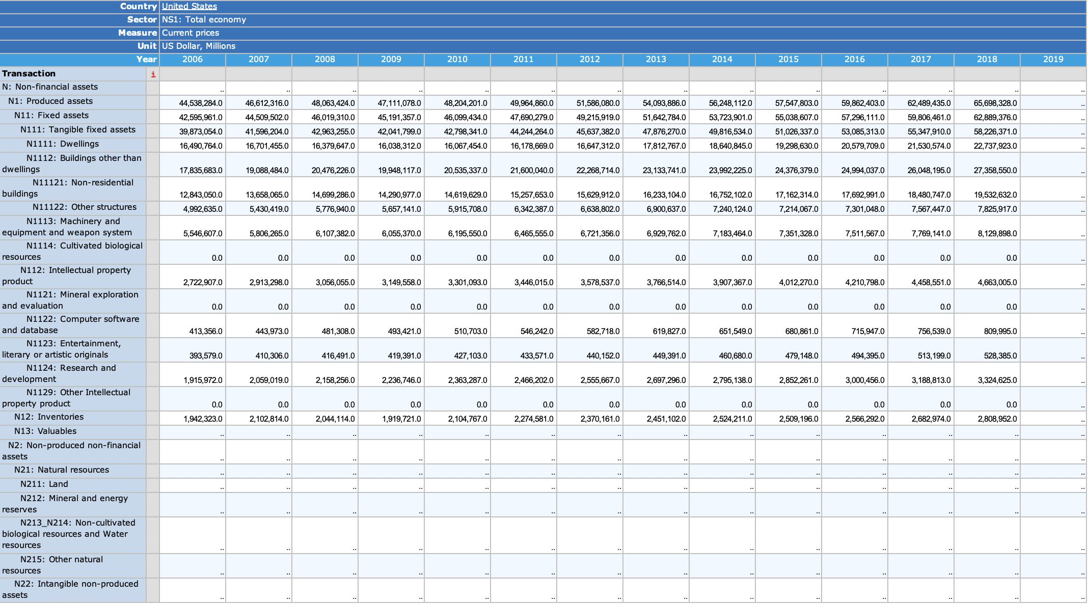
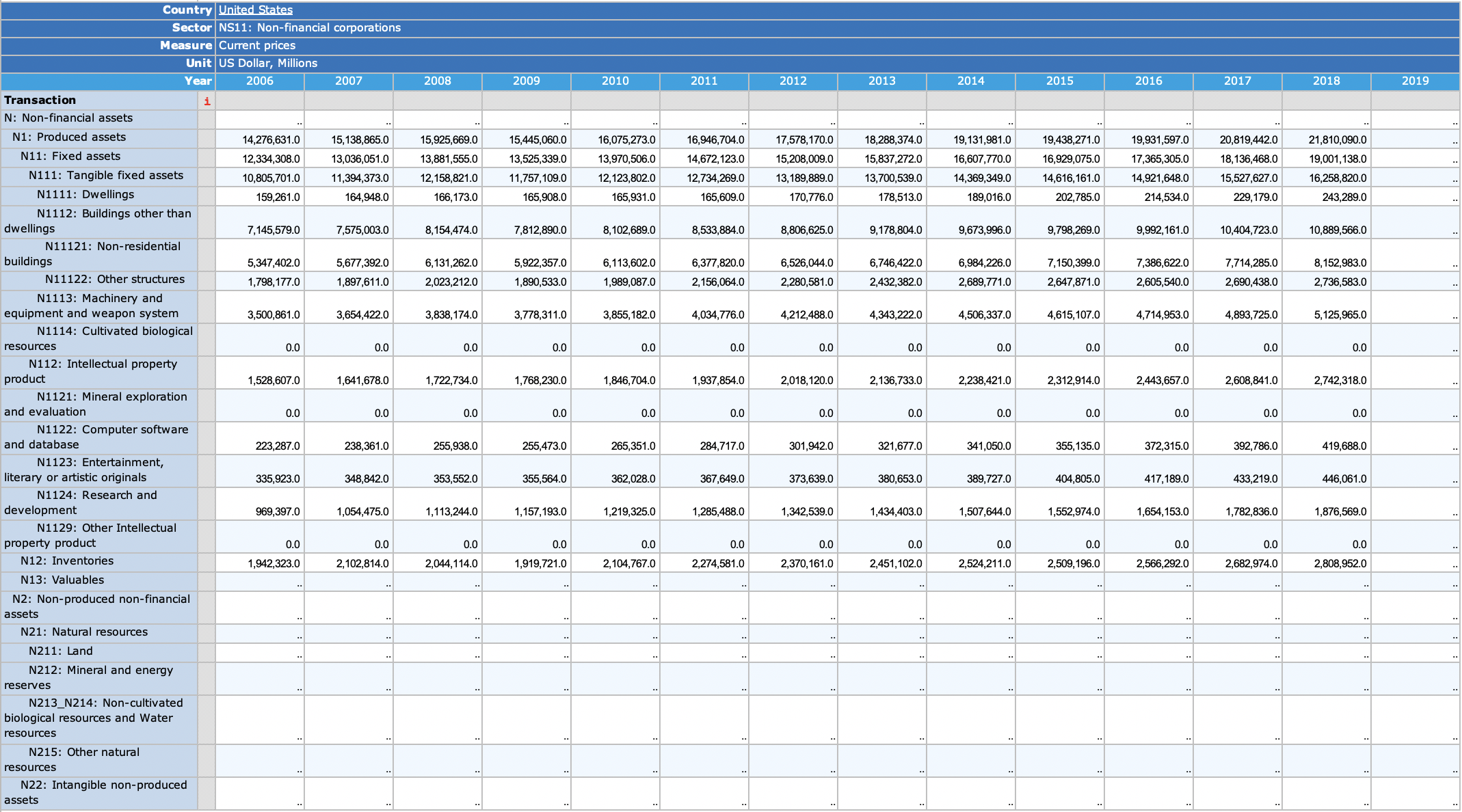
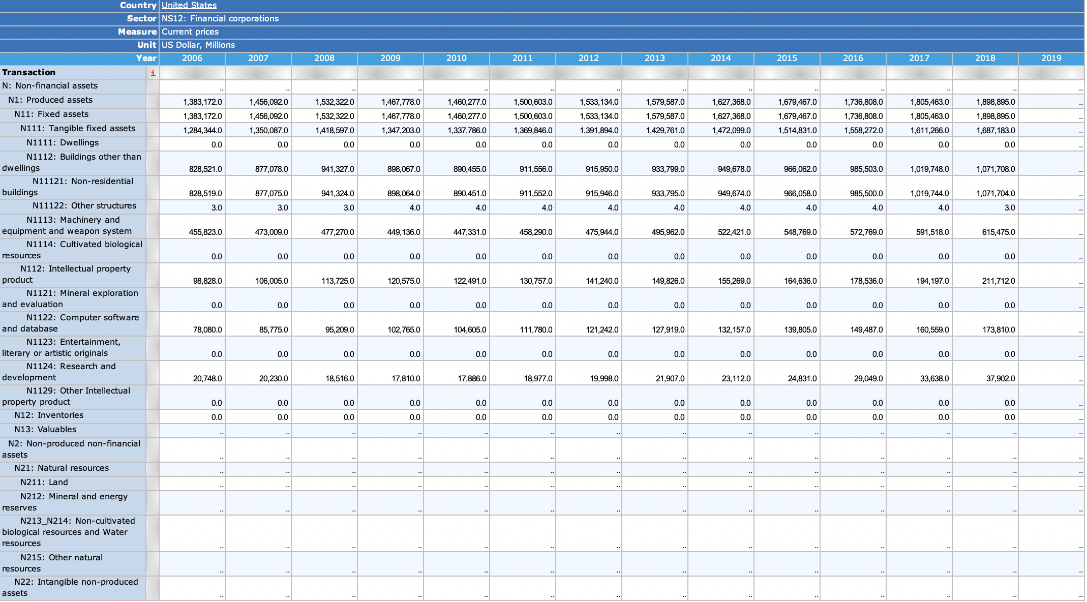
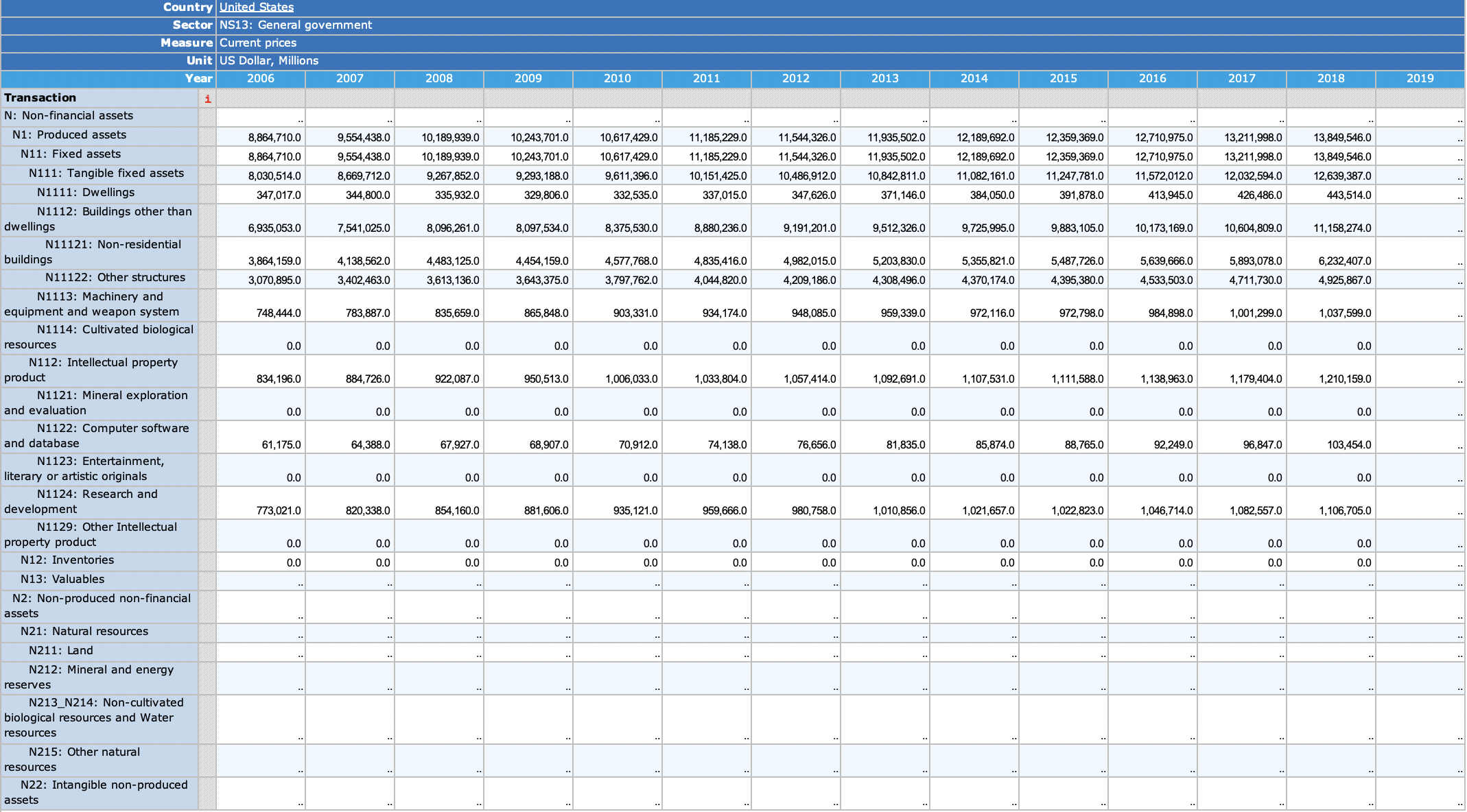
{if (is_html_output()) datatable(., filter = 'top', rownames = F, escape = F) else .}United States
Code
SNA_TABLE9B %>%
  filter(LOCATION == "USA",
         obsTime == "2018",
         SECTOR %in% c("NS1", "NS11", "NS12", "NS13", "NS14_S15")) %>%
  left_join(SNA_TABLE9B_var$TRANSACT, by = "TRANSACT") %>%
  left_join(SNA_TABLE1 %>%
              filter(TRANSACT == "B1_GE",
                     MEASURE == "C") %>%
              select(obsTime, LOCATION, B1_GE = obsValue),
            by = c("LOCATION", "obsTime")) %>%
  mutate(obsValue = round(100*obsValue / B1_GE, 1) %>% paste0(., "%")) %>%
  select(SECTOR, TRANSACT, Transact, obsValue) %>%
  mutate(SECTOR = gsub("N", "", SECTOR),
         SECTOR = paste0('<img src="../../icon/sector/vsmall/', SECTOR, '.png" alt="All">')) %>%
  spread(SECTOR, obsValue) %>%
  {if (is_html_output()) datatable(., filter = 'top', rownames = F, escape = F) else .}
New Zealand
Code
SNA_TABLE9B %>%
  filter(LOCATION == "NZL",
         obsTime == "2017",
         SECTOR %in% c("NS1", "NS11", "NS12", "NS13", "NS14_S15")) %>%
  left_join(SNA_TABLE9B_var$TRANSACT, by = "TRANSACT") %>%
  left_join(SNA_TABLE1 %>%
              filter(TRANSACT == "B1_GE",
                     MEASURE == "C") %>%
              select(obsTime, LOCATION, B1_GE = obsValue),
            by = c("LOCATION", "obsTime")) %>%
  mutate(obsValue = round(100*obsValue / B1_GE, 1) %>% paste0(., "%")) %>%
  select(SECTOR, TRANSACT, Transact, obsValue) %>%
  mutate(SECTOR = gsub("N", "", SECTOR),
         SECTOR = paste0('<img src="../../icon/sector/vsmall/', SECTOR, '.png" alt="All">')) %>%
  spread(SECTOR, obsValue) %>%
  {if (is_html_output()) datatable(., filter = 'top', rownames = F, escape = F) else .}
Australia
Code
SNA_TABLE9B %>%
  filter(LOCATION == "AUS",
         obsTime == "2017",
         SECTOR %in% c("NS1", "NS11", "NS12", "NS13", "NS14_S15")) %>%
  left_join(SNA_TABLE9B_var$TRANSACT, by = "TRANSACT") %>%
  left_join(SNA_TABLE1 %>%
              filter(TRANSACT == "B1_GE",
                     MEASURE == "C") %>%
              select(obsTime, LOCATION, B1_GE = obsValue),
            by = c("LOCATION", "obsTime")) %>%
  mutate(obsValue = round(100*obsValue / B1_GE, 1) %>% paste0(., "%")) %>%
  select(SECTOR, TRANSACT, Transact, obsValue) %>%
  mutate(SECTOR = gsub("N", "", SECTOR),
         SECTOR = paste0('<img src="../../icon/sector/vsmall/', SECTOR, '.png" alt="All">')) %>%
  spread(SECTOR, obsValue) %>%
  {if (is_html_output()) datatable(., filter = 'top', rownames = F, escape = F) else .}
Canada
Code
SNA_TABLE9B %>%
  filter(LOCATION == "CAN",
         obsTime == "2018",
         SECTOR %in% c("NS1", "NS11", "NS12", "NS13", "NS14_S15")) %>%
  left_join(SNA_TABLE9B_var$TRANSACT, by = "TRANSACT") %>%
  left_join(SNA_TABLE1 %>%
              filter(TRANSACT == "B1_GE",
                     MEASURE == "C") %>%
              select(obsTime, LOCATION, B1_GE = obsValue),
            by = c("LOCATION", "obsTime")) %>%
  mutate(obsValue = round(100*obsValue / B1_GE, 1) %>% paste0(., "%")) %>%
  select(SECTOR, TRANSACT, Transact, obsValue) %>%
  mutate(SECTOR = gsub("N", "", SECTOR),
         SECTOR = paste0('<img src="../../icon/sector/vsmall/', SECTOR, '.png" alt="All">')) %>%
  spread(SECTOR, obsValue) %>%
  {if (is_html_output()) datatable(., filter = 'top', rownames = F, escape = F) else .}
Germany
Code
SNA_TABLE9B %>%
  filter(LOCATION == "DEU",
         obsTime == "2018",
         SECTOR %in% c("NS1", "NS11", "NS12", "NS13", "NS14_S15")) %>%
  left_join(SNA_TABLE9B_var$TRANSACT, by = "TRANSACT") %>%
  left_join(SNA_TABLE1 %>%
              filter(TRANSACT == "B1_GE",
                     MEASURE == "C") %>%
              select(obsTime, LOCATION, B1_GE = obsValue),
            by = c("LOCATION", "obsTime")) %>%
  mutate(obsValue = round(100*obsValue / B1_GE, 1) %>% paste0(., "%")) %>%
  select(SECTOR, TRANSACT, Transact, obsValue) %>%
  mutate(SECTOR = gsub("N", "", SECTOR),
         SECTOR = paste0('<img src="../../icon/sector/vsmall/', SECTOR, '.png" alt="All">')) %>%
  spread(SECTOR, obsValue) %>%
  {if (is_html_output()) datatable(., filter = 'top', rownames = F, escape = F) else .}
Japan
Code
SNA_TABLE9B %>%
  filter(LOCATION == "JPN",
         obsTime == "2018",
         SECTOR %in% c("NS1", "NS11", "NS12", "NS13", "NS14_S15")) %>%
  left_join(SNA_TABLE9B_var$TRANSACT, by = "TRANSACT") %>%
  left_join(SNA_TABLE1 %>%
              filter(TRANSACT == "B1_GE",
                     MEASURE == "C") %>%
              select(obsTime, LOCATION, B1_GE = obsValue),
            by = c("LOCATION", "obsTime")) %>%
  mutate(obsValue = round(100*obsValue / B1_GE, 1) %>% paste0(., "%")) %>%
  select(SECTOR, TRANSACT, Transact, obsValue) %>%
  mutate(SECTOR = gsub("N", "", SECTOR),
         SECTOR = paste0('<img src="../../icon/sector/vsmall/', SECTOR, '.png" alt="All">')) %>%
  spread(SECTOR, obsValue) %>%
  {if (is_html_output()) datatable(., filter = 'top', rownames = F, escape = F) else .}
Czech Republic
Code
SNA_TABLE9B %>%
  filter(LOCATION == "CZE",
         obsTime == "2018",
         SECTOR %in% c("NS1", "NS11", "NS12", "NS13", "NS14_S15")) %>%
  left_join(SNA_TABLE9B_var$TRANSACT, by = "TRANSACT") %>%
  left_join(SNA_TABLE1 %>%
              filter(TRANSACT == "B1_GE",
                     MEASURE == "C") %>%
              select(obsTime, LOCATION, B1_GE = obsValue),
            by = c("LOCATION", "obsTime")) %>%
  mutate(obsValue = round(100*obsValue / B1_GE, 1) %>% paste0(., "%")) %>%
  select(SECTOR, TRANSACT, Transact, obsValue) %>%
  mutate(SECTOR = gsub("N", "", SECTOR),
         SECTOR = paste0('<img src="../../icon/sector/vsmall/', SECTOR, '.png" alt="All">')) %>%
  spread(SECTOR, obsValue) %>%
  {if (is_html_output()) datatable(., filter = 'top', rownames = F, escape = F) else .}
N2 - Non-produced assets
Table
Code
SNA_TABLE9B %>%
filter(TRANSACT == "N2",
SECTOR %in% c("NS1", "NS11", "NS12", "NS13", "NS14_S15")) %>%
group_by(LOCATION, SECTOR) %>%
summarise(obsValue = last(obsValue),
obsTime = last(obsTime)) %>%
left_join(SNA_TABLE1 %>%
filter(TRANSACT == "B1_GE",
MEASURE == "C") %>%
select(obsTime, LOCATION, B1_GE = obsValue),
by = c("LOCATION", "obsTime")) %>%
select(-obsTime) %>%
mutate(obsValue = round(100*obsValue / B1_GE, 1) %>% paste0(., "%"),
SECTOR = gsub("N", "", SECTOR)) %>%
ungroup %>%
left_join(SNA_TABLE9B_var$LOCATION, by = "LOCATION") %>%
select(LOCATION, Location, SECTOR, obsValue) %>%
mutate(Flag = gsub(" ", "-", str_to_lower(Location)),
Flag = paste0('<img src="../../icon/flag/vsmall/', Flag, '.png" alt="Flag">')) %>%
select(Flag, everything()) %>%
mutate(SECTOR = paste0('<img src="../../icon/sector/vsmall/', SECTOR, '.png" alt="All">')) %>%
spread(SECTOR, obsValue) %>%
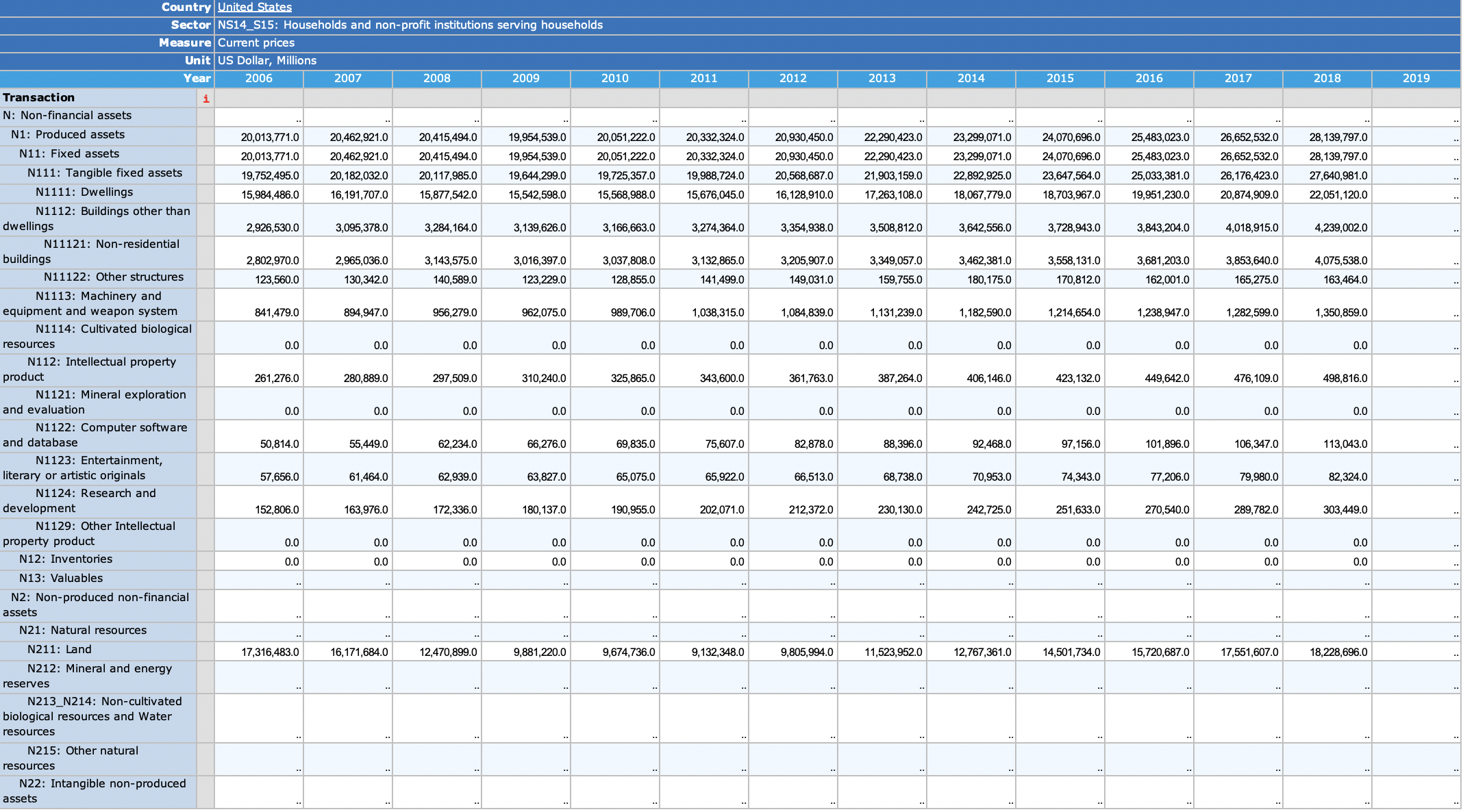
{if (is_html_output()) datatable(., filter = 'top', rownames = F, escape = F) else .}United States, France, Germany, Japan, Canada, Australia
Code
load_data("oecd/SNA_TABLE9B_var2.RData")
SNA_TABLE9B %>%
  filter(LOCATION %in% c("FRA", "USA", "DEU", "GBR", "ITA", "ESP", "CAN", "JPN", "AUS"),
         SECTOR == "NS1",
         TRANSACT %in% c("N211")) %>%
  left_join(SNA_TABLE9B_var$LOCATION, by = "LOCATION") %>%
  left_join(SNA_TABLE1 %>%
              filter(TRANSACT == "B1_GE",
                     MEASURE == "C") %>%
              select(obsTime, LOCATION, B1_GE = obsValue),
            by = c("LOCATION", "obsTime")) %>%
  mutate(obsValue = obsValue / B1_GE) %>%
  year_to_date %>%
  select(LOCATION, Location, date, obsValue) %>%
  left_join(colors, by = c("Location" = "country")) %>%
  ggplot + theme_minimal() + ylab("% of GDP") + xlab("") + add_6flags + scale_color_identity() +
  geom_line(aes(x = date, y = obsValue, color = color)) +
  scale_y_continuous(breaks = 0.01*seq(0, 1300, 100),
                     labels = scales::percent_format(accuracy = 1)) +
  scale_x_date(breaks = seq(1920, 2025, 5) %>% paste0("-01-01") %>% as.Date,
               labels = date_format("%Y"))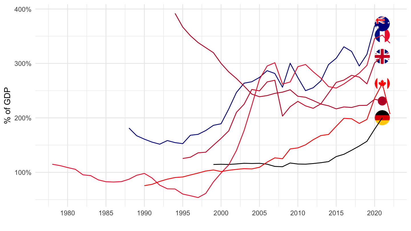
Czech Republic, Hungary, Korea, Mexico, New Zealand, Norway, Sweden
Code
load_data("oecd/SNA_TABLE9B_var2.RData")
SNA_TABLE9B %>%
  filter(LOCATION %in% c("CZE", "HUN", "KOR", "MEX", "NZL", "NOR", "SWE"),
         SECTOR == "NS1",
         TRANSACT %in% c("N211")) %>%
  left_join(SNA_TABLE9B_var$LOCATION, by = "LOCATION") %>%
  left_join(SNA_TABLE1 %>%
              filter(TRANSACT == "B1_GE",
                     MEASURE == "C") %>%
              select(obsTime, LOCATION, B1_GE = obsValue),
            by = c("LOCATION", "obsTime")) %>%
  mutate(obsValue = obsValue / B1_GE) %>%
  year_to_date %>%
  select(LOCATION, Location, date, obsValue) %>%
  left_join(colors, by = c("Location" = "country")) %>%
  ggplot + theme_minimal() + ylab("% of GDP") + xlab("") + add_6flags + scale_color_identity() +
  geom_line(aes(x = date, y = obsValue, color = color)) +
  scale_y_continuous(breaks = 0.01*seq(0, 1300, 100),
                     labels = scales::percent_format(accuracy = 1)) +
  scale_x_date(breaks = seq(1920, 2025, 5) %>% paste0("-01-01") %>% as.Date,
               labels = date_format("%Y"))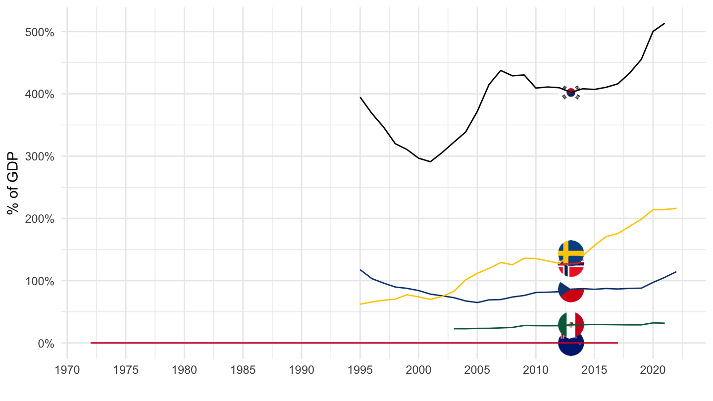
Time Series
France
Code
SNA_TABLE9B %>%
  filter(LOCATION == "FRA",
         SECTOR == "NS1",
         TRANSACT %in% c("N", "N1", "N2")) %>%
  left_join(SNA_TABLE9B_var$TRANSACT, by = "TRANSACT") %>%
  left_join(SNA_TABLE1 %>%
              filter(TRANSACT == "B1_GE",
                     MEASURE == "C") %>%
              select(obsTime, LOCATION, B1_GE = obsValue),
            by = c("LOCATION", "obsTime")) %>%
  mutate(obsValue = obsValue / B1_GE) %>%
  year_to_date %>%
  select(TRANSACT, Transact, date, obsValue) %>%
  ggplot + theme_minimal() + ylab("% of GDP") + xlab("") +
  geom_line(aes(x = date, y = obsValue, color = Transact, linetype = Transact)) +
  scale_y_continuous(breaks = 0.01*seq(0, 1300, 100),
                     labels = scales::percent_format(accuracy = 1),
                     limits = c(0, 8)) +
  scale_x_date(breaks = seq(1920, 2025, 5) %>% paste0("-01-01") %>% as.Date,
               labels = date_format("%Y")) +

  theme(legend.position = c(0.3, 0.85),
        legend.title = element_blank())
United Kingdom
Code
SNA_TABLE9B %>%
  filter(LOCATION == "GBR",
         SECTOR == "NS1",
         TRANSACT %in% c("N", "N1", "N2")) %>%
  left_join(SNA_TABLE9B_var$TRANSACT, by = "TRANSACT") %>%
  left_join(SNA_TABLE1 %>%
              filter(TRANSACT == "B1_GE",
                     MEASURE == "C") %>%
              select(obsTime, LOCATION, B1_GE = obsValue),
            by = c("LOCATION", "obsTime")) %>%
  mutate(obsValue = obsValue / B1_GE) %>%
  year_to_date %>%
  select(TRANSACT, Transact, date, obsValue) %>%
  ggplot + theme_minimal() + ylab("% of GDP") + xlab("") +
  geom_line(aes(x = date, y = obsValue, color = Transact, linetype = Transact)) +
  scale_y_continuous(breaks = 0.01*seq(0, 1300, 100),
                     labels = scales::percent_format(accuracy = 1),
                     limits = c(0, 6)) +
  scale_x_date(breaks = seq(1920, 2025, 2) %>% paste0("-01-01") %>% as.Date,
               labels = date_format("%Y")) +

  theme(legend.position = c(0.2, 0.9),
        legend.title = element_blank())
Japan
Code
SNA_TABLE9B %>%
  filter(LOCATION == "JPN",
         SECTOR == "NS1",
         TRANSACT %in% c("N", "N1", "N2")) %>%
  left_join(SNA_TABLE9B_var$TRANSACT, by = "TRANSACT") %>%
  left_join(SNA_TABLE1 %>%
              filter(TRANSACT == "B1_GE",
                     MEASURE == "C") %>%
              select(obsTime, LOCATION, B1_GE = obsValue),
            by = c("LOCATION", "obsTime")) %>%
  mutate(obsValue = obsValue / B1_GE) %>%
  year_to_date %>%
  select(TRANSACT, Transact, date, obsValue) %>%
  ggplot + theme_minimal() + ylab("% of GDP") + xlab("") +
  geom_line(aes(x = date, y = obsValue, color = Transact, linetype = Transact)) +
  scale_y_continuous(breaks = 0.01*seq(0, 1300, 100),
                     labels = scales::percent_format(accuracy = 1),
                     limits = c(0, 9)) +
  scale_x_date(breaks = seq(1920, 2025, 5) %>% paste0("-01-01") %>% as.Date,
               labels = date_format("%Y")) +

  theme(legend.position = c(0.7, 0.9),
        legend.title = element_blank())
Fixed Assets: K/L Substitution
U.S.
Code
SNA_TABLE9B %>%
  filter(TRANSACT %in% c("N1111", "B1_GE", "N1112", "N1113", "N112", "N12"),
         SECTOR == "NS1",
         LOCATION == "USA") %>%
  left_join(SNA_TABLE9B_var$TRANSACT, by = "TRANSACT") %>%
  year_to_date %>%
  select(date, Transact, obsValue) %>%
  spread(Transact, obsValue) %>%
  mutate_at(vars(-`Gross domestic product (expenditure approach)`, -date), funs(./ `Gross domestic product (expenditure approach)`)) %>%
  select(-`Gross domestic product (expenditure approach)`) %>%
  gather(Transact, value, -date) %>%
  ggplot(.) + theme_minimal() + xlab("") + ylab("Fixed Assets (% of GDP)") +
  geom_line(aes(x = date, y = value, color = Transact)) +
  theme(legend.position = c(0.7, 0.5),
        legend.title = element_blank(),
        legend.text = element_text(size = 8),
        legend.key.size = unit(0.9, 'lines')) +

  scale_y_continuous(breaks = 0.01*seq(0, 500, 20),
                     labels = scales::percent_format(accuracy = 1)) +
  scale_x_date(breaks = seq(1700, 2020, 5) %>% paste0(., "-01-01") %>% as.Date,
               limits =  c(1970, 2018) %>% paste0(., "-01-01") %>% as.Date,
               labels = date_format("%Y"))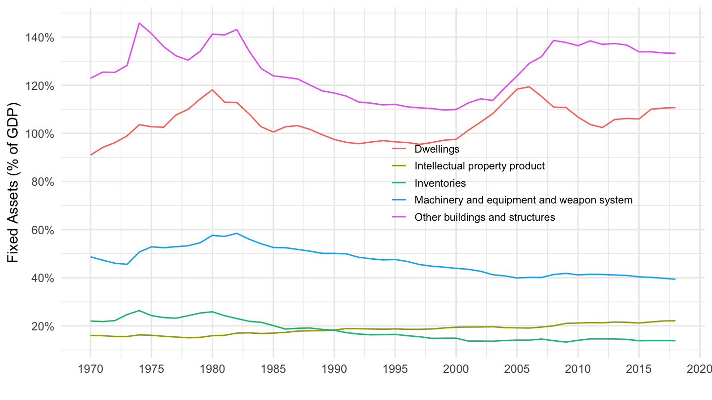
France
Code
SNA_TABLE9B %>%
  filter(TRANSACT %in% c("N1111", "B1_GE", "N1112", "N1113", "N112", "N12"),
         SECTOR == "NS1",
         LOCATION == "FRA") %>%
  left_join(SNA_TABLE9B_var$TRANSACT, by = "TRANSACT") %>%
  year_to_date %>%
  select(date, Transact, obsValue) %>%
  spread(Transact, obsValue) %>%
  mutate_at(vars(-`Gross domestic product (expenditure approach)`, -date), funs(./ `Gross domestic product (expenditure approach)`)) %>%
  select(-`Gross domestic product (expenditure approach)`) %>%
  gather(Transact, value, -date) %>%
  na.omit %>%
  ggplot(.) + geom_line(aes(x = date, y = value, color = Transact)) +
  theme_minimal() +
  theme(legend.position = c(0.3, 0.90),
        legend.title = element_blank(),
        legend.text = element_text(size = 8),
        legend.key.size = unit(0.9, 'lines')) +

  scale_y_continuous(breaks = 0.01*seq(0, 500, 20),
                     labels = scales::percent_format(accuracy = 1)) +
  scale_x_date(breaks = seq(1700, 2020, 5) %>% paste0(., "-01-01") %>% as.Date,
               labels = date_format("%Y")) +
  xlab("") + ylab("Fixed Assets (% of GDP)")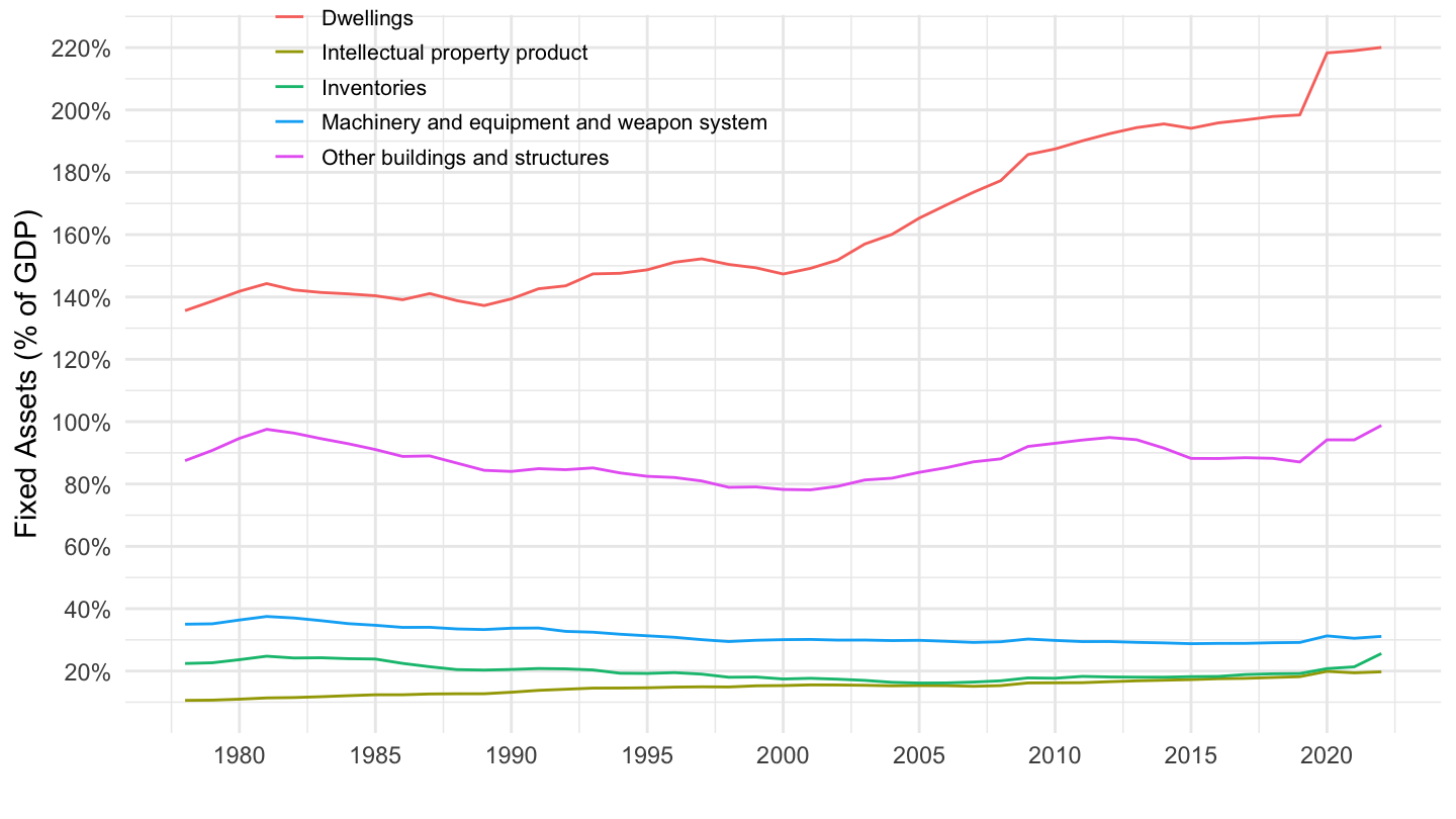
Germany
Code
SNA_TABLE9B %>%
  filter(TRANSACT %in% c("N1111", "B1_GE", "N1112", "N1113", "N112", "N12"),
         SECTOR == "NS1",
         LOCATION == "DEU") %>%
  left_join(SNA_TABLE9B_var$TRANSACT, by = "TRANSACT") %>%
  year_to_date %>%
  select(date, Transact, obsValue) %>%
  spread(Transact, obsValue) %>%
  mutate_at(vars(-`Gross domestic product (expenditure approach)`, -date), funs(./ `Gross domestic product (expenditure approach)`)) %>%
  select(-`Gross domestic product (expenditure approach)`) %>%
  gather(Transact, value, -date) %>%
  na.omit %>%
  ggplot(.) + geom_line(aes(x = date, y = value, color = Transact)) +
  theme_minimal() +
  theme(legend.position = c(0.4, 0.50),
        legend.title = element_blank(),
        legend.text = element_text(size = 8),
        legend.key.size = unit(0.9, 'lines')) +

  scale_y_continuous(breaks = 0.01*seq(0, 500, 20),
                     labels = scales::percent_format(accuracy = 1)) +
  scale_x_date(breaks = seq(1700, 2020, 1) %>% paste0(., "-01-01") %>% as.Date,
               labels = date_format("%Y")) +
  xlab("") + ylab("Fixed Assets (% of GDP)")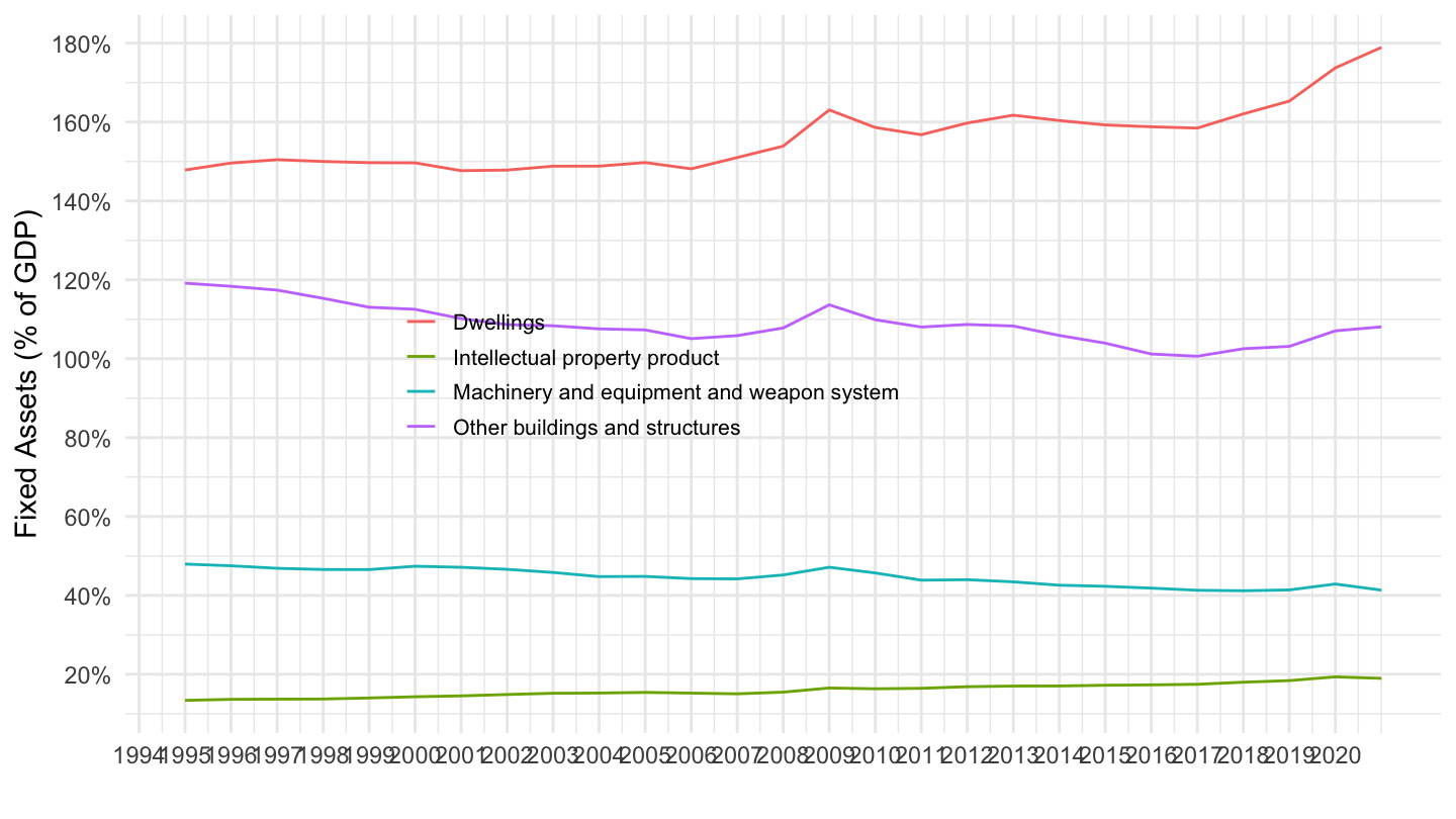
United Kingdom
Code
SNA_TABLE9B %>%
  filter(TRANSACT %in% c("N1111", "B1_GE", "N1112", "N1113", "N112", "N12"),
         SECTOR == "NS1",
         LOCATION == "GBR") %>%
  left_join(SNA_TABLE9B_var$TRANSACT, by = "TRANSACT") %>%
  year_to_date %>%
  select(date, Transact, obsValue) %>%
  spread(Transact, obsValue) %>%
  mutate_at(vars(-`Gross domestic product (expenditure approach)`, -date), funs(./ `Gross domestic product (expenditure approach)`)) %>%
  select(-`Gross domestic product (expenditure approach)`) %>%
  gather(Transact, value, -date) %>%
  na.omit %>%
  ggplot(.) + geom_line(aes(x = date, y = value, color = Transact)) +
  theme_minimal() +
  theme(legend.position = c(0.4, 0.50),
        legend.title = element_blank(),
        legend.text = element_text(size = 8),
        legend.key.size = unit(0.9, 'lines')) +

  scale_y_continuous(breaks = 0.01*seq(0, 500, 20),
                     labels = scales::percent_format(accuracy = 1)) +
  scale_x_date(breaks = seq(1700, 2020, 1) %>% paste0(., "-01-01") %>% as.Date,
               labels = date_format("%Y")) +
  xlab("") + ylab("Fixed Assets (% of GDP)")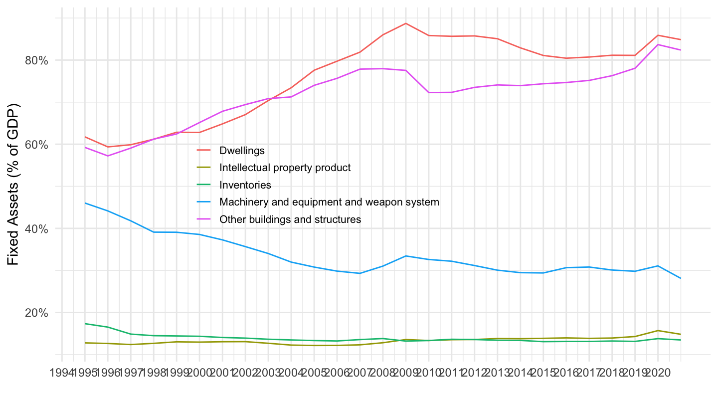
SNA_TABLE9B_ex1
png
Code
i_g("bib/oecd/SNA_TABLE9B_ex1.png")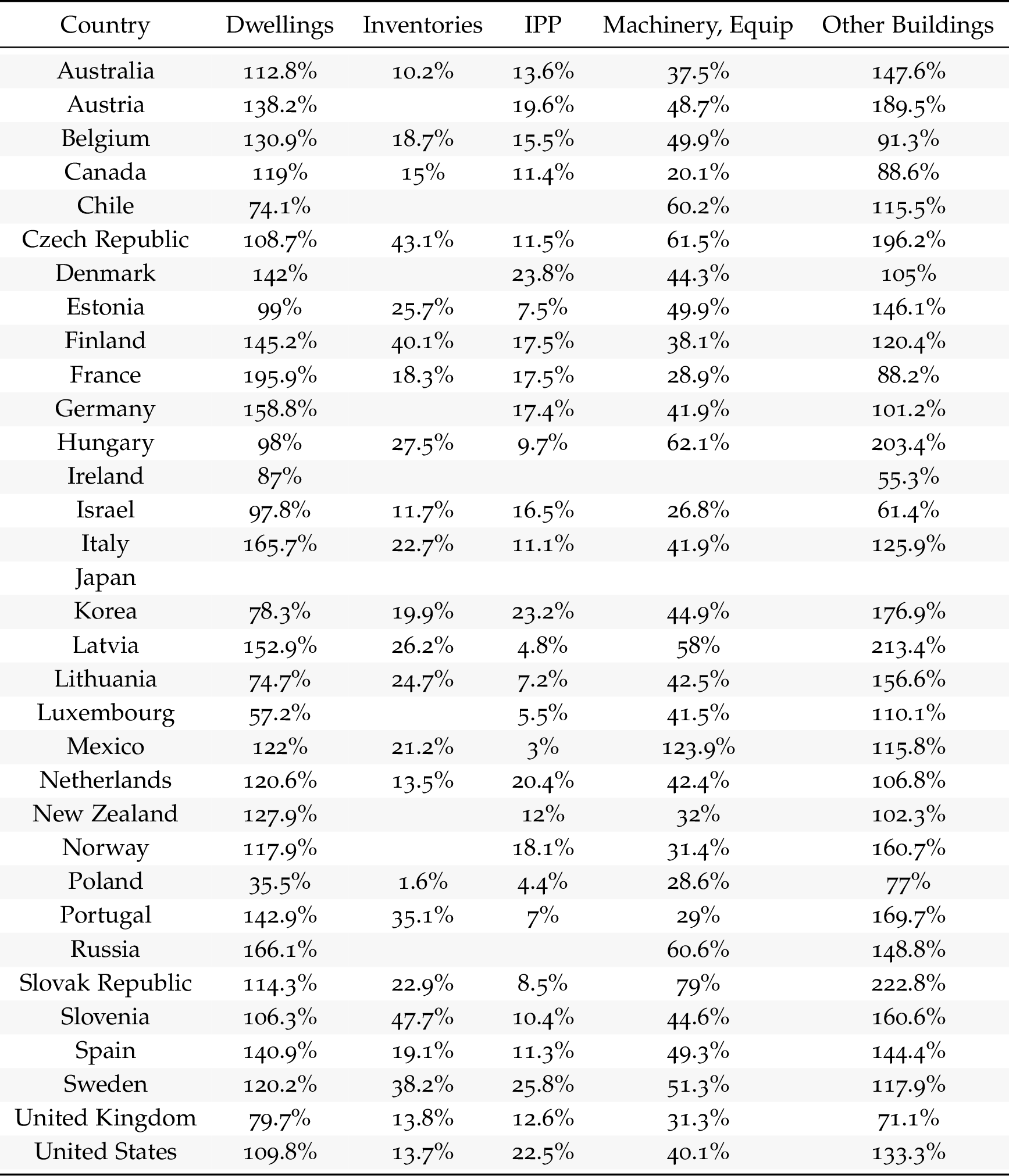
Code
| Location | Dwellings | Inventories | IPP | Machinery, Equip | Other Buildings |
|---|---|---|---|---|---|
| Australia | 113% | 10.1% | 13.6% | 37.6% | 147.9% |
| Austria | 138.1% | 29.5% | 19.6% | 48.7% | 189.5% |
| Belgium | 130.9% | 18.7% | 15.5% | 49.9% | 91.3% |
| Canada | 119% | 15.4% | 11.4% | 20.1% | 88.6% |
| Chile | 76.4% | 45.4% | 149.5% | ||
| Croatia | 127.5% | 28.5% | 12.5% | 59.1% | 241% |
| Czech Republic | 108.7% | 43.1% | 11.5% | 61.5% | 196.2% |
| Denmark | 142% | 14.9% | 23.8% | 44.3% | 105% |
| Estonia | 99.9% | 24.8% | 7.6% | 50.8% | 147.9% |
| Finland | 145.2% | 40.1% | 17.5% | 38.1% | 120.4% |
| France | 195.9% | 18.3% | 17.5% | 28.9% | 88.2% |
| Germany | 158.8% | 17.3% | 41.8% | 101.2% | |
| Greece | 159.5% | 19.2% | 4.9% | 51.1% | 96.5% |
| Hungary | 97.9% | 27.7% | 9.9% | 61.6% | 204.4% |
| Ireland | 88.3% | 114.6% | 47.1% | 55.4% | |
| Israel | 101.4% | 12.2% | 17.9% | 33% | 68.7% |
| Italy | 165.7% | 22.7% | 11.1% | 41.9% | 126% |
| Japan | |||||
| Korea | 78.3% | 19.9% | 23.2% | 44.9% | 176.9% |
| Latvia | 153% | 25.9% | 4.7% | 58.2% | 214.9% |
| Lithuania | 74.7% | 24.7% | 7.2% | 42.5% | 156.6% |
| Luxembourg | 55.6% | 4.9% | 39.1% | 113.3% | |
| Mexico | 121.9% | 21.1% | 3% | 123.9% | 115.7% |
| Netherlands | 120.6% | 13.5% | 20.4% | 42.4% | 106.8% |
| New Zealand | 127.4% | 11.9% | 31.9% | 101.9% | |
| Norway | 117.4% | 18% | 30.9% | 159.9% | |
| Poland | 35.7% | 1.7% | 4.4% | 28.8% | 77.4% |
| Portugal | 142.9% | 35.1% | 7% | 29% | 169.7% |
| Romania | 50.2% | 41.9% | 8.6% | 133.1% | 153.9% |
| Russia | 166.1% | 60.6% | 148.8% | ||
| Slovak Republic | 114% | 22.8% | 8.6% | 79% | 222.3% |
| Slovenia | 106.3% | 47.7% | 10.4% | 44.7% | 160.6% |
| Spain | 140.9% | 19.1% | 11.3% | 49.2% | 144.4% |
| Sweden | 122.1% | 38.2% | 25.9% | 50% | 117.8% |
| United Kingdom | 80.4% | 13.1% | 14% | 30.7% | 74.7% |
| United States | 110% | 13.9% | 21.6% | 40.2% | 133.9% |
SNA_TABLE9B_ex2
png
Code
i_g("bib/oecd/SNA_TABLE9B_ex2.png")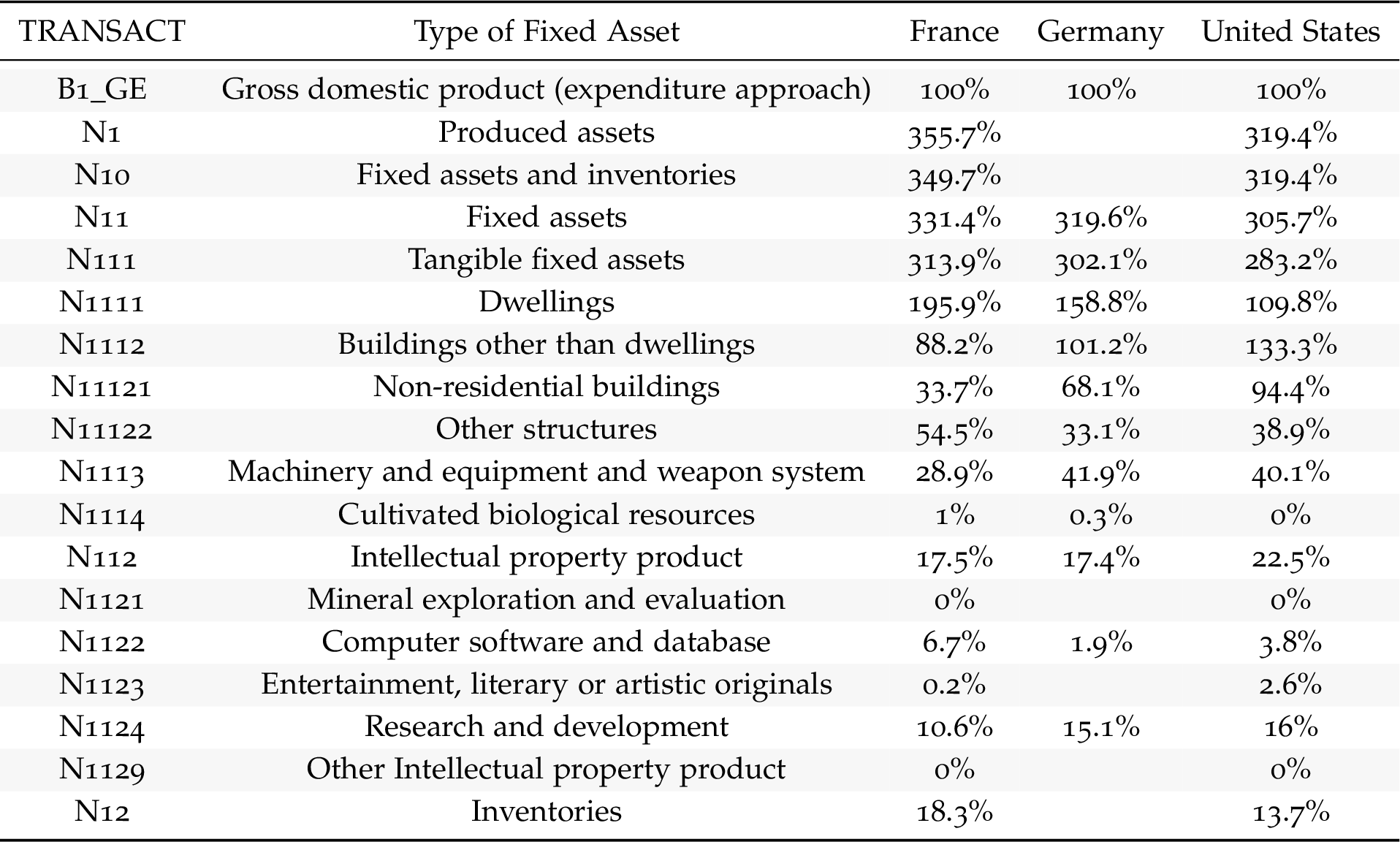
Code
| TRANSACT | Transact | France | Germany | United States |
|---|---|---|---|---|
| B1_GE | Gross domestic product (expenditure approach) | 100% | 100% | 100% |
| N1 | Produced assets | 355.7% | 320.2% | |
| N10 | Fixed assets and inventories | 349.7% | 319.6% | |
| N11 | Fixed assets | 331.4% | 319.5% | 305.7% |
| N111 | Tangible fixed assets | 313.9% | 302.1% | 284.1% |
| N1111 | Dwellings | 195.9% | 158.8% | 110% |
| N1112 | Other buildings and structures | 88.2% | 101.2% | 133.9% |
| N11121 | Buildings other than dwellings | 33.7% | 68.1% | 94.8% |
| N11122 | Other structures | 54.5% | 33.1% | 39.1% |
| N1113 | Machinery and equipment and weapon system | 28.9% | 41.8% | 40.2% |
| N1114 | Cultivated biological resources | 1% | 0.3% | 0% |
| N112 | Intellectual property product | 17.5% | 17.3% | 21.6% |
| N1121 | Mineral exploration and evaluation | 0% | 0% | |
| N1122 | Computer software and database | 6.7% | 1.9% | 3.9% |
| N1123 | Entertainment, literary or artistic originals | 0.2% | 2.6% | |
| N1124 | Research and development | 10.6% | 15% | 15.1% |
| N1129 | Other Intellectual property product | 0% | 0% | |
| N12 | Inventories | 18.3% | 13.9% |