Value added and its components by activity, ISIC rev4, SNA93 - SNA_TABLE6A_SNA93
Data - OECD
Nobs
Data Structure
| id | description |
|---|---|
| LOCATION | Country |
| TRANSACT | Transaction |
| ACTIVITY | Activity |
| MEASURE | Measure |
| TIME | Year |
| OBS_VALUE | Observation Value |
| TIME_FORMAT | Time Format |
| OBS_STATUS | Observation Status |
| UNIT | Unit |
| POWERCODE | Unit multiplier |
| REFERENCEPERIOD | Reference period |
LOCATION
TRANSACT
| id | label |
|---|---|
| P1A | Output |
| VA4 | 6A--Value added and its components by activity, ISIC rev4 |
| P2A | Intermediate consumption |
| D1A | Compensation of employees |
| B1GA | Gross value added |
| D11A | of which: gross wages and salaries |
| K1A | Consumption of fixed capital |
| B2G_B3GA | Gross operating surplus and gross mixed income |
| B1_GE | Gross domestic product (expenditure approach) |
| B2N_B3NA | Net operating surplus and net mixed income |
| D29_D39A | Other taxes less other subsidies on production |
ACTIVITY
MEASURE
| id | label |
|---|---|
| C | Current prices |
| V | Constant prices, national base year |
| VOB | Constant prices, OECD base year |
TIME_FORMAT
| id | label |
|---|---|
| P1Y | Annual |
| P1M | Monthly |
| P3M | Quarterly |
| P6M | Half-yearly |
| P1D | Daily |
Ex 1A: VA in Manuf.
Code
SNA_TABLE6A_SNA93 %>%
filter(TRANSACT %in% c("B1GA", "B1_GE"),
ACTIVITY %in% c("VC", "VTOT"),
MEASURE == "C") %>%
left_join(SNA_TABLE6A_SNA93_var %>% pluck("LOCATION"), by = c("LOCATION" = "id")) %>%
rename(LOCATION_desc = label) %>%
year_to_date %>%
mutate(VARIABLE = paste0(TRANSACT, "_", ACTIVITY)) %>%
select(VARIABLE, LOCATION, LOCATION_desc, date, obsValue) %>%
spread(VARIABLE, obsValue) %>%
mutate(value = B1GA_VC / B1_GE_VTOT) %>%
filter(!is.na(value)) %>%
group_by(LOCATION, LOCATION_desc) %>%
summarise(year1 = first(year(date)),
value1 = first(value),
year2 = last(year(date)),
value2 = last(value)) %>%
mutate_at(vars(value1, value2), funs(paste0(round(100*., digits = 1), " %"))) %>%
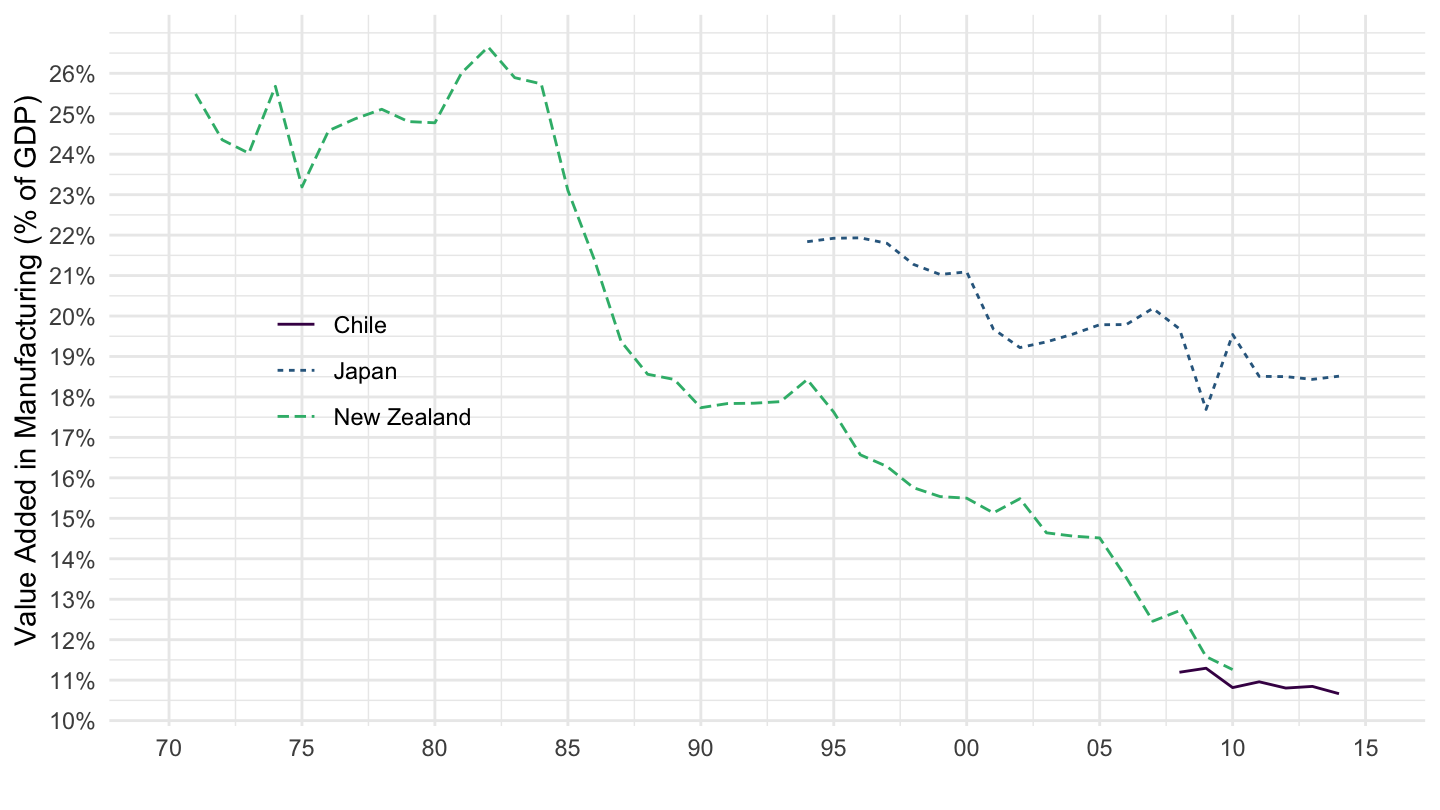
{if (is_html_output()) datatable(., filter = 'top', rownames = F) else .}Ex 1B: VA in Manuf. (Chile, Japan, New Zealand)
Code
SNA_TABLE6A_SNA93 %>%
  filter(TRANSACT %in% c("B1GA", "B1_GE"),
         ACTIVITY %in% c("VC", "VTOT"),
         LOCATION %in% c("JPN", "CHL", "NZL"),
         MEASURE == "C") %>%
  left_join(SNA_TABLE6A_SNA93_var %>% pluck("LOCATION"), by = c("LOCATION" = "id")) %>%
  rename(LOCATION_desc = label) %>%
  year_to_date %>%
  mutate(VARIABLE = paste0(TRANSACT, "_", ACTIVITY)) %>%
  select(VARIABLE, LOCATION_desc, date, obsValue) %>%
  spread(VARIABLE, obsValue) %>%
  mutate(value = B1GA_VC / B1_GE_VTOT) %>%
  ggplot() +
  geom_line(aes(x = date, y = value, color = LOCATION_desc, linetype = LOCATION_desc)) +
  scale_color_manual(values = viridis(4)[1:3]) +
  theme_minimal() +
  scale_x_date(breaks = seq(1920, 2100, 5) %>% paste0("-01-01") %>% as.Date,
               labels = date_format("%Y")) +
  theme(legend.position = c(0.2, 0.5),
        legend.title = element_blank()) +
  scale_y_continuous(breaks = 0.01*seq(-7, 26, 1),
                     labels = scales::percent_format(accuracy = 1)) +
  ylab("Value Added in Manufacturing (% of GDP)") + xlab("")