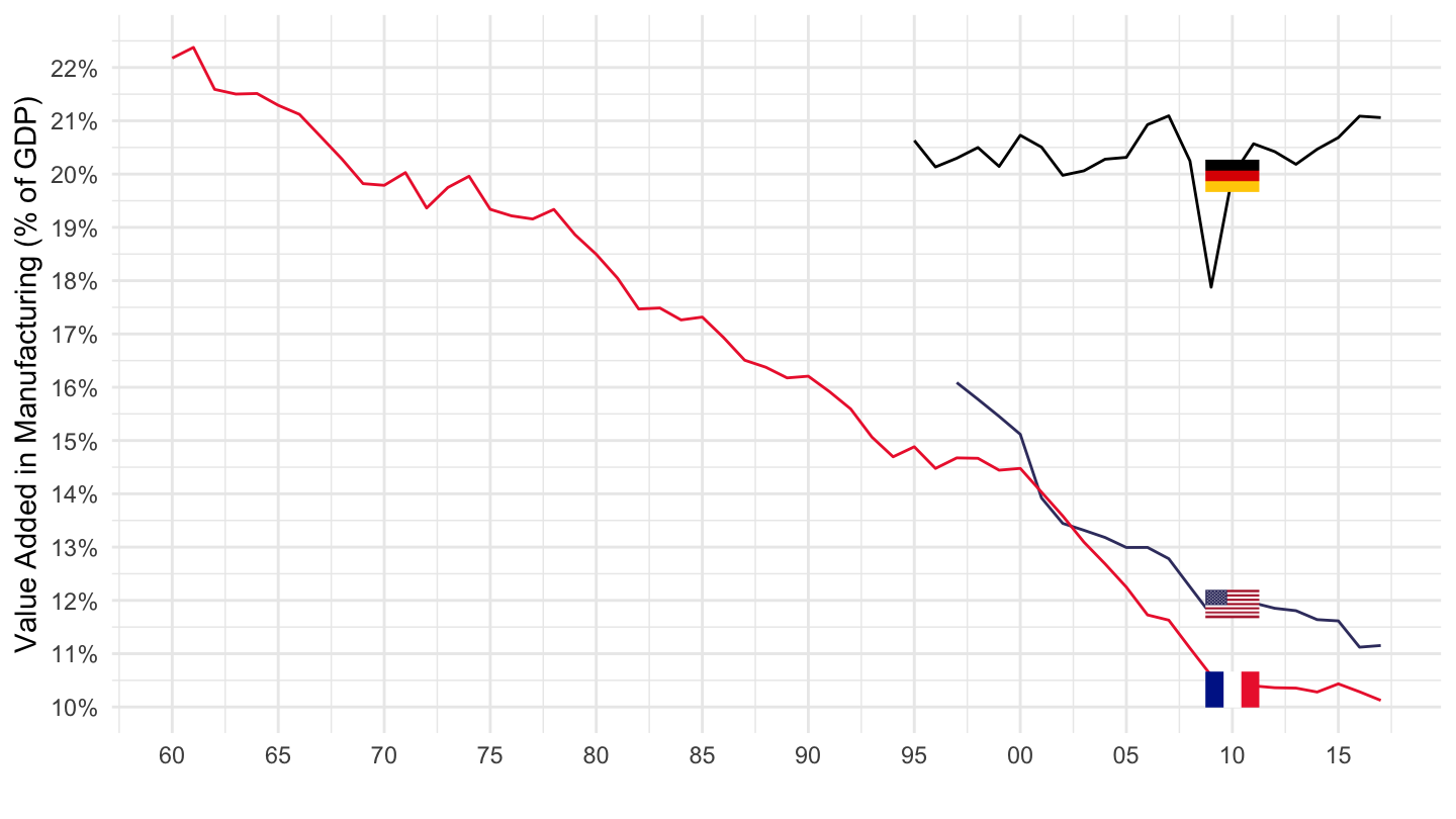
SNA_TABLE6A_ARCHIVE %>%
  filter(TRANSACT %in% c("B1GA", "B1_GE"),
         ACTIVITY %in% c("VC", "VTOT"),
         LOCATION %in% c("FRA", "DEU", "USA"),
         MEASURE == "C") %>%
  left_join(SNA_TABLE6A_ARCHIVE_var$LOCATION, by = "LOCATION") %>%
  year_to_date %>%
  mutate(VARIABLE = paste0(TRANSACT, "_", ACTIVITY)) %>%
  select(VARIABLE, Location, date, obsValue) %>%
  spread(VARIABLE, obsValue) %>%
  mutate(obsValue = B1GA_VC / B1_GE_VTOT) %>%
  na.omit %>%
  left_join(colors, by = c("Location" = "country")) %>%
  ggplot(.) + geom_line(aes(x = date, y = obsValue, color = color)) +
  scale_color_identity() + add_3flags + theme_minimal() +
  scale_x_date(breaks = seq(1920, 2100, 5) %>% paste0("-01-01") %>% as.Date,
               labels = date_format("%Y")) +
  theme(legend.position = c(0.2, 0.5),
        legend.title = element_blank()) +
  scale_y_continuous(breaks = 0.01*seq(-7, 26, 1),
                     labels = scales::percent_format(accuracy = 1)) +
  ylab("Value Added in Manufacturing (% of GDP)") + xlab("")