Disposable income and net lending - net borrowing, 2019 archive - SNA_TABLE2_ARCHIVE
Data - OECD
Layout
- OECD Website. html
Nobs - Javascript
Code
SNA_TABLE2_ARCHIVE %>%
  left_join(SNA_TABLE2_ARCHIVE_var %>% pluck("TRANSACT"), by = c("TRANSACT" = "id")) %>%
  rename(`TRANSACT Description` = label) %>%
  group_by(TRANSACT, `TRANSACT Description`, MEASURE) %>%
  summarise(nobs = n()) %>%
  arrange(-nobs) %>%
  {if (is_html_output()) datatable(., filter = 'top', rownames = F) else .}
TRANSACT
Code
SNA_TABLE2_ARCHIVE %>%
  left_join(SNA_TABLE2_ARCHIVE_var %>% pluck("TRANSACT"), by = c("TRANSACT" = "id")) %>%
  rename(`TRANSACT Description` = label) %>%
  group_by(TRANSACT, `TRANSACT Description`) %>%
  summarise(Nobs = n()) %>%
  arrange(-Nobs) %>%
  {if (is_html_output()) datatable(., filter = 'top', rownames = F) else .}
MEASURE
Code
SNA_TABLE2_ARCHIVE %>%
  left_join(SNA_TABLE2_ARCHIVE_var %>% pluck("MEASURE"), by = c("MEASURE" = "id")) %>%
  rename(`MEASURE Description` = label) %>%
  group_by(MEASURE, `MEASURE Description`) %>%
  summarise(Nobs = n()) %>%
  arrange(-Nobs) %>%
  {if (is_html_output()) datatable(., filter = 'top', rownames = F) else .}
B1_GE - Gross domestic product
All Decomposition
Code
SNA_TABLE2_ARCHIVE %>%
  filter(LOCATION %in% c("FRA", "DEU", "USA", "GBR"),
         obsTime == "2018",
         MEASURE == "C") %>%
  select(LOCATION, TRANSACT, obsValue) %>%
  left_join(SNA_TABLE2_ARCHIVE_var$TRANSACT %>%
              setNames(c("TRANSACT", "TRANSACT_desc")), by = "TRANSACT") %>%
  spread(LOCATION, obsValue) %>%
  mutate_at(vars(-1, -2), funs(paste0(round(100*./.[TRANSACT == "B1_GE"], 1), " %"))) %>%
  {if (is_html_output()) datatable(., filter = 'top', rownames = F) else .}
How much data
Code
SNA_TABLE2_ARCHIVE %>%
  filter(TRANSACT == "B1_GE",
         MEASURE == "C") %>%
  left_join(SNA_TABLE2_ARCHIVE_var$LOCATION %>%
              setNames(c("LOCATION", "LOCATION_desc")),
            by = "LOCATION") %>%
  group_by(LOCATION, UNIT, LOCATION_desc) %>%
  summarise(year_first = first(obsTime),
            year_last = last(obsTime),
            value_last = last(round(obsValue))) %>%
  {if (is_html_output()) datatable(., filter = 'top', rownames = F) else .}
All
US and France
Code
SNA_TABLE2_ARCHIVE %>%
  filter(obsTime == "2018",
         MEASURE == "C",
         LOCATION %in% c("USA", "FRA")) %>%
  select(LOCATION, TRANSACT, obsValue) %>%
  left_join(SNA_TABLE2_ARCHIVE_var$TRANSACT %>%
              setNames(c("TRANSACT", "TRANSACT_desc")), by = "TRANSACT") %>%
  spread(LOCATION, obsValue) %>%
  mutate_at(vars(-1, -2), funs(paste0(round(100*./.[TRANSACT == "B1_GE"], 1), " %"))) %>%
{if (is_html_output()) print_table(.) else .}| TRANSACT | TRANSACT_desc | FRA | USA |
|---|---|---|---|
| B1_GE | Gross domestic product (expenditure approach) | 100 % | 100 % |
B8NS1 - Net Saving / GDP
France, Germany, Italy
Code
SNA_TABLE2_ARCHIVE %>%
  filter(MEASURE == "C",
         LOCATION %in% c("FRA", "DEU", "ITA"),
         TRANSACT %in% c("B1_GE", "B8NS1")) %>%
  year_to_enddate %>%
  left_join(SNA_TABLE2_ARCHIVE_var$LOCATION %>%
              setNames(c("LOCATION", "LOCATION_desc")), by = "LOCATION") %>%
  select(LOCATION_desc, date, TRANSACT, obsValue) %>%
  spread(TRANSACT, obsValue) %>%
  group_by(LOCATION_desc) %>%
  mutate(B8NS1_B1_GE = B8NS1 / B1_GE) %>%
  select(LOCATION_desc, date, B8NS1_B1_GE) %>%
  na.omit %>%
  ggplot() + geom_line(aes(x = date, y = B8NS1_B1_GE, color = LOCATION_desc, linetype = LOCATION_desc)) +
  scale_color_manual(values = viridis(4)[1:3]) +
  theme_minimal() +
  scale_x_date(breaks = seq(1920, 2100, 10) %>% paste0("-01-01") %>% as.Date,
               labels = date_format("%Y")) +
  theme(legend.position = c(0.85, 0.9),
        legend.title = element_blank()) +
  scale_y_continuous(breaks = 0.01*seq(-10, 100, 1),
                     labels = scales::percent_format(accuracy = 1)) +
  ylab("Net Saving (% of GDP)") + xlab("")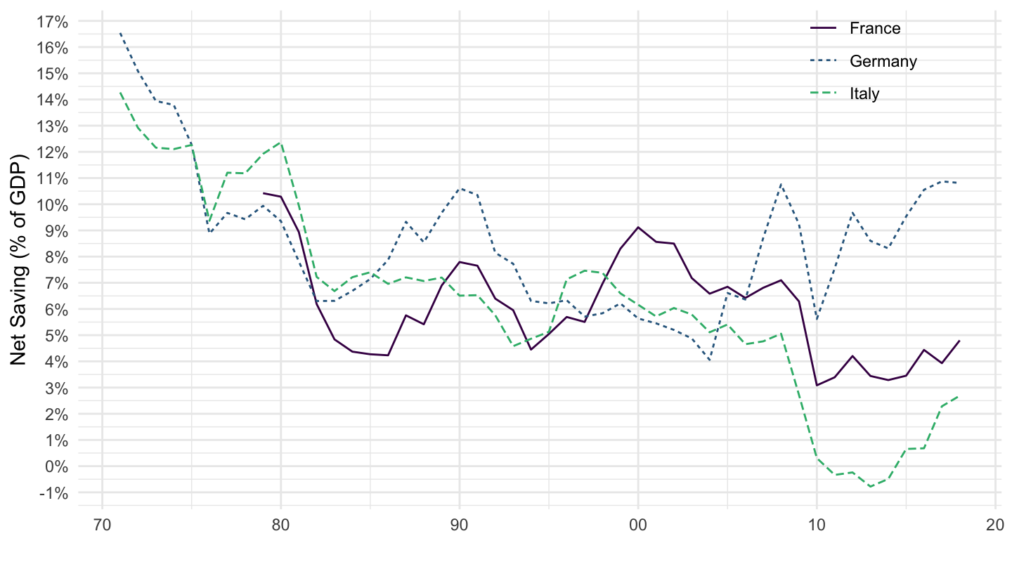
France, Italy
Code
SNA_TABLE2_ARCHIVE %>%
  filter(MEASURE == "C",
         LOCATION %in% c("FRA", "ITA"),
         TRANSACT %in% c("B1_GE", "B8NS1")) %>%
  year_to_enddate %>%
  left_join(SNA_TABLE2_ARCHIVE_var$LOCATION %>%
              setNames(c("LOCATION", "LOCATION_desc")), by = "LOCATION") %>%
  select(LOCATION_desc, date, TRANSACT, obsValue) %>%
  spread(TRANSACT, obsValue) %>%
  group_by(LOCATION_desc) %>%
  mutate(B8NS1_B1_GE = B8NS1 / B1_GE) %>%
  select(LOCATION_desc, date, B8NS1_B1_GE) %>%
  na.omit %>%
  ggplot() + geom_line(aes(x = date, y = B8NS1_B1_GE, color = LOCATION_desc, linetype = LOCATION_desc)) +
  scale_color_manual(values = viridis(4)[1:3]) +
  theme_minimal() +
  scale_x_date(breaks = seq(1920, 2100, 10) %>% paste0("-01-01") %>% as.Date,
               labels = date_format("%Y")) +
  theme(legend.position = c(0.85, 0.9),
        legend.title = element_blank()) +
  scale_y_continuous(breaks = 0.01*seq(-10, 100, 1),
                     labels = scales::percent_format(accuracy = 1)) +
  ylab("Net Saving (% of GDP)") + xlab("")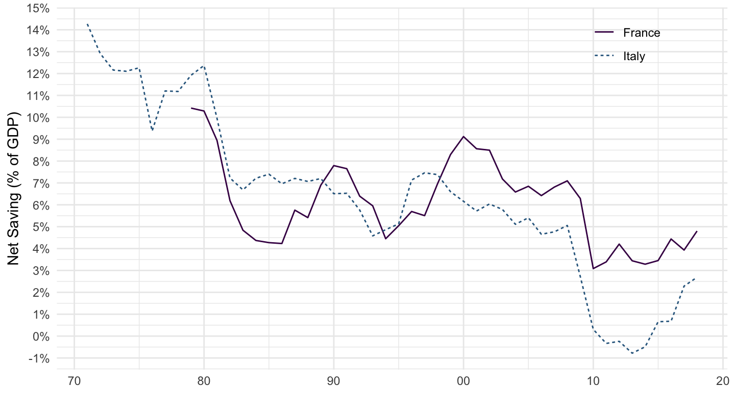
United Kingdom, Japan, United States
Code
SNA_TABLE2_ARCHIVE %>%
  filter(MEASURE == "C",
         LOCATION %in% c("JPN", "GBR", "USA"),
         TRANSACT %in% c("B1_GE", "B8NS1")) %>%
  year_to_enddate %>%
  left_join(SNA_TABLE2_ARCHIVE_var$LOCATION %>%
              setNames(c("LOCATION", "LOCATION_desc")), by = "LOCATION") %>%
  select(LOCATION_desc, date, TRANSACT, obsValue) %>%
  spread(TRANSACT, obsValue) %>%
  group_by(LOCATION_desc) %>%
  mutate(B8NS1_B1_GE = B8NS1 / B1_GE) %>%
  select(LOCATION_desc, date, B8NS1_B1_GE) %>%
  na.omit %>%
  ggplot() + geom_line(aes(x = date, y = B8NS1_B1_GE, color = LOCATION_desc, linetype = LOCATION_desc)) +
  scale_color_manual(values = viridis(4)[1:3]) +
  theme_minimal() +
  scale_x_date(breaks = seq(1920, 2100, 10) %>% paste0("-01-01") %>% as.Date,
               labels = date_format("%Y")) +
  theme(legend.position = c(0.85, 0.9),
        legend.title = element_blank()) +
  scale_y_continuous(breaks = 0.01*seq(-10, 100, 1),
                     labels = scales::percent_format(accuracy = 1)) +
  ylab("Net Saving (% of GDP)") + xlab("")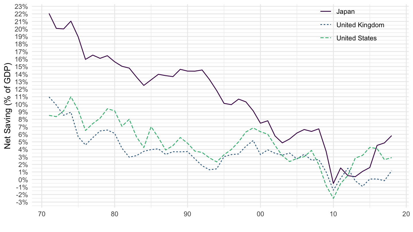
Switzerland, Germany, Netherlands
Code
SNA_TABLE2_ARCHIVE %>%
  filter(MEASURE == "C",
         LOCATION %in% c("NLD", "CHE", "DEU"),
         TRANSACT %in% c("B1_GE", "B8NS1")) %>%
  year_to_enddate %>%
  left_join(SNA_TABLE2_ARCHIVE_var$LOCATION %>%
              setNames(c("LOCATION", "LOCATION_desc")), by = "LOCATION") %>%
  select(LOCATION_desc, date, TRANSACT, obsValue) %>%
  spread(TRANSACT, obsValue) %>%
  group_by(LOCATION_desc) %>%
  mutate(B8NS1_B1_GE = B8NS1 / B1_GE) %>%
  select(LOCATION_desc, date, B8NS1_B1_GE) %>%
  na.omit %>%
  ggplot() + theme_minimal() +
  geom_line(aes(x = date, y = B8NS1_B1_GE, color = LOCATION_desc, linetype = LOCATION_desc)) +
  scale_color_manual(values = viridis(4)[1:3]) +
  scale_x_date(breaks = seq(1920, 2100, 10) %>% paste0("-01-01") %>% as.Date,
               labels = date_format("%Y")) +
  theme(legend.position = c(0.35, 0.8),
        legend.title = element_blank()) +
  scale_y_continuous(breaks = 0.01*seq(-10, 100, 2),
                     labels = scales::percent_format(accuracy = 1)) +
  ylab("Net Saving (% of GDP)") + xlab("")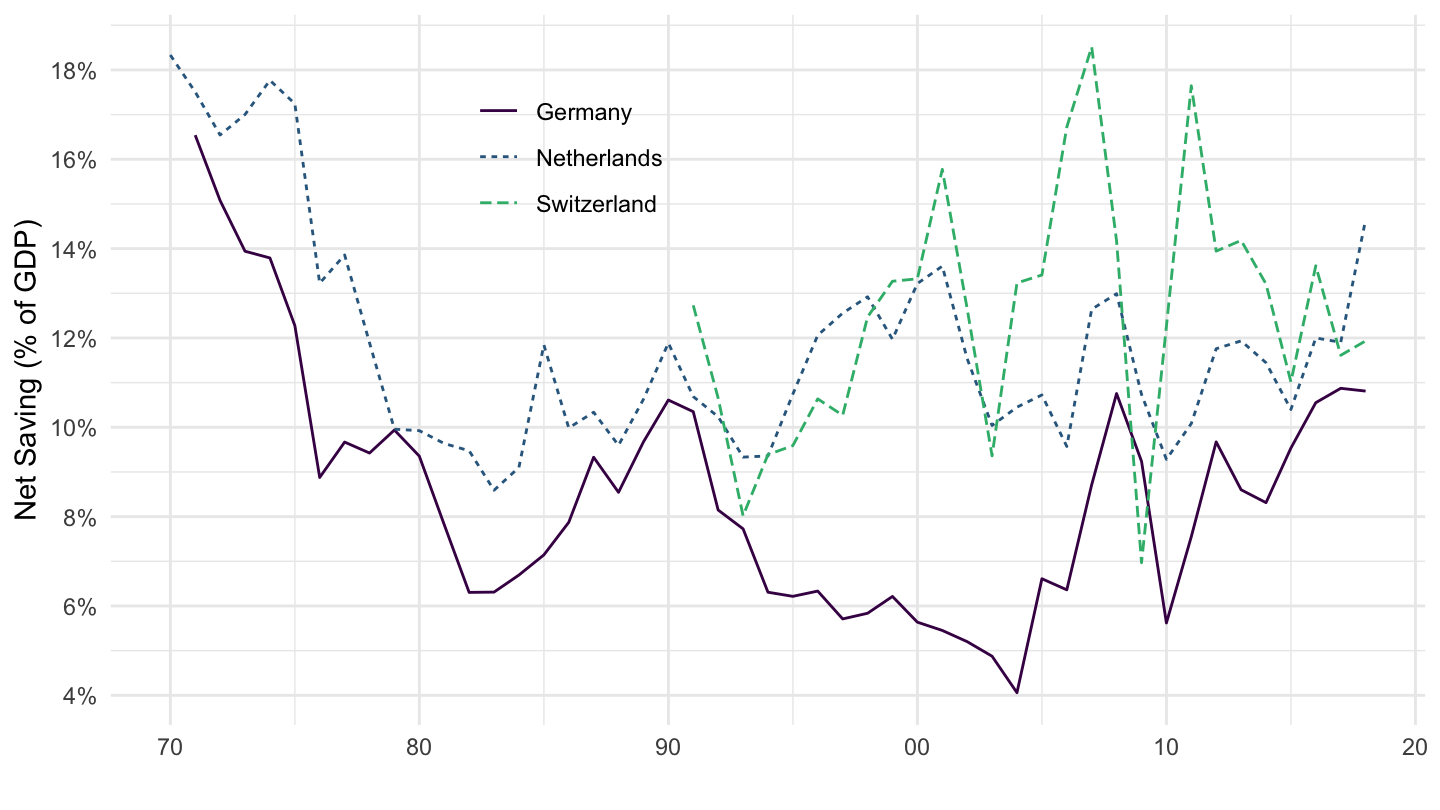
B9S1 - Net Saving / GDP
France, Germany, Italy
Code
SNA_TABLE2_ARCHIVE %>%
  filter(MEASURE == "C",
         LOCATION %in% c("FRA", "DEU", "ITA"),
         TRANSACT %in% c("B1_GE", "B9S1")) %>%
  year_to_enddate %>%
  left_join(SNA_TABLE2_ARCHIVE_var$LOCATION %>%
              setNames(c("LOCATION", "LOCATION_desc")), by = "LOCATION") %>%
  select(LOCATION_desc, date, TRANSACT, obsValue) %>%
  spread(TRANSACT, obsValue) %>%
  group_by(LOCATION_desc) %>%
  mutate(value = B9S1 / B1_GE) %>%
  select(LOCATION_desc, date, value) %>%
  na.omit %>%
  ggplot() + geom_line(aes(x = date, y = value, color = LOCATION_desc, linetype = LOCATION_desc)) +
  scale_color_manual(values = viridis(4)[1:3]) +
  theme_minimal() +
  scale_x_date(breaks = seq(1920, 2100, 10) %>% paste0("-01-01") %>% as.Date,
               labels = date_format("%Y")) +
  theme(legend.position = c(0.85, 0.9),
        legend.title = element_blank()) +
  scale_y_continuous(breaks = 0.01*seq(-10, 100, 1),
                     labels = scales::percent_format(accuracy = 1)) +
  ylab("Net Saving (% of GDP)") + xlab("")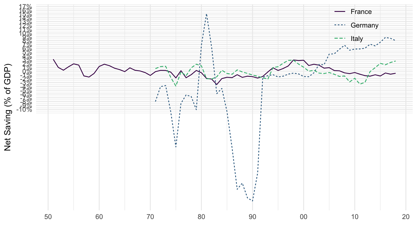
France, Germany, Italy
Code
SNA_TABLE2_ARCHIVE %>%
  filter(MEASURE == "C",
         LOCATION %in% c("FRA", "ITA"),
         TRANSACT %in% c("B1_GE", "B9S1")) %>%
  year_to_enddate %>%
  left_join(SNA_TABLE2_ARCHIVE_var$LOCATION %>%
              setNames(c("LOCATION", "LOCATION_desc")), by = "LOCATION") %>%
  select(LOCATION_desc, date, TRANSACT, obsValue) %>%
  spread(TRANSACT, obsValue) %>%
  group_by(LOCATION_desc) %>%
  mutate(value = B9S1 / B1_GE) %>%
  select(LOCATION_desc, date, value) %>%
  na.omit %>%
  ggplot() + geom_line(aes(x = date, y = value, color = LOCATION_desc, linetype = LOCATION_desc)) +
  scale_color_manual(values = viridis(4)[1:3]) +
  theme_minimal() +
  scale_x_date(breaks = seq(1920, 2100, 10) %>% paste0("-01-01") %>% as.Date,
               labels = date_format("%Y")) +
  theme(legend.position = c(0.85, 0.9),
        legend.title = element_blank()) +
  scale_y_continuous(breaks = 0.01*seq(-10, 100, 1),
                     labels = scales::percent_format(accuracy = 1)) +
  ylab("Net Saving (% of GDP)") + xlab("")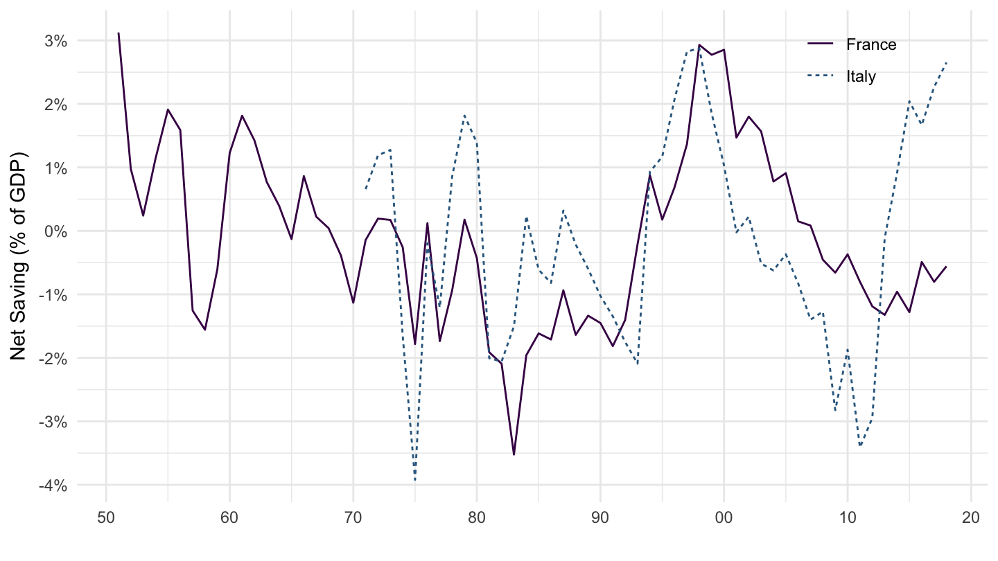
United Kingdom, Japan, United States
Code
SNA_TABLE2_ARCHIVE %>%
  filter(MEASURE == "C",
         LOCATION %in% c("JPN", "GBR", "USA"),
         TRANSACT %in% c("B1_GE", "B9S1")) %>%
  year_to_enddate %>%
  left_join(SNA_TABLE2_ARCHIVE_var$LOCATION %>%
              setNames(c("LOCATION", "LOCATION_desc")), by = "LOCATION") %>%
  select(LOCATION_desc, date, TRANSACT, obsValue) %>%
  spread(TRANSACT, obsValue) %>%
  group_by(LOCATION_desc) %>%
  mutate(value = B9S1 / B1_GE) %>%
  select(LOCATION_desc, date, value) %>%
  na.omit %>%
  ggplot() + geom_line(aes(x = date, y = value, color = LOCATION_desc, linetype = LOCATION_desc)) +
  scale_color_manual(values = viridis(4)[1:3]) +
  theme_minimal() +
  scale_x_date(breaks = seq(1920, 2100, 10) %>% paste0("-01-01") %>% as.Date,
               labels = date_format("%Y")) +
  theme(legend.position = c(0.85, 0.9),
        legend.title = element_blank()) +
  scale_y_continuous(breaks = 0.01*seq(-10, 100, 1),
                     labels = scales::percent_format(accuracy = 1)) +
  ylab("Net Saving (% of GDP)") + xlab("")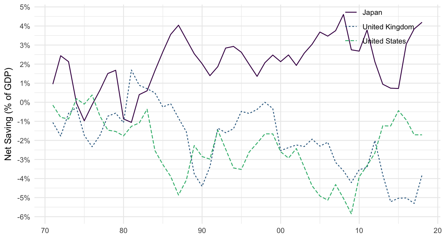
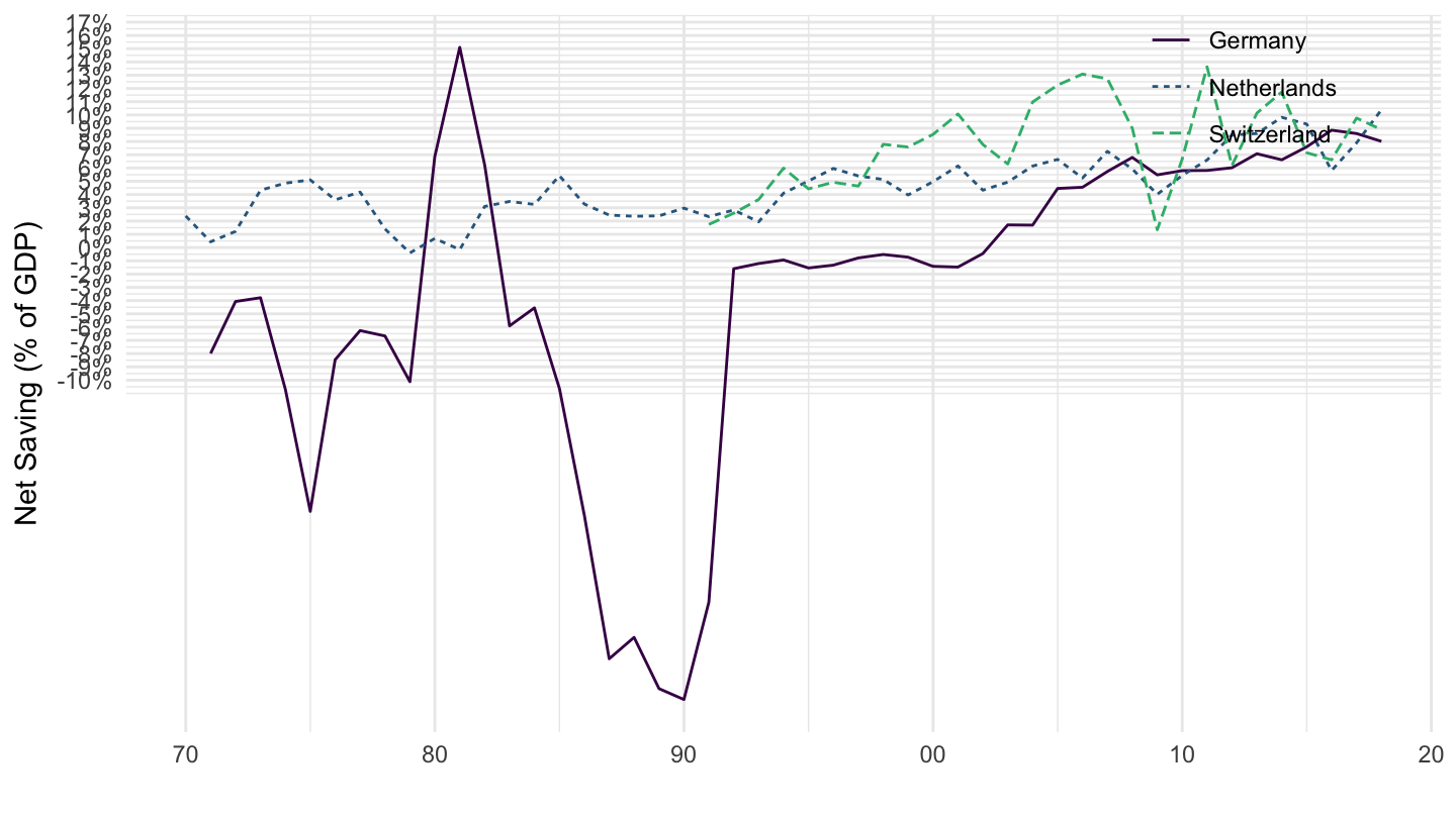
Switzerland, Germany, Netherlands
Code
SNA_TABLE2_ARCHIVE %>%
  filter(MEASURE == "C",
         LOCATION %in% c("NLD", "CHE", "DEU"),
         TRANSACT %in% c("B1_GE", "B9S1")) %>%
  year_to_enddate %>%
  left_join(SNA_TABLE2_ARCHIVE_var$LOCATION %>%
              setNames(c("LOCATION", "LOCATION_desc")), by = "LOCATION") %>%
  select(LOCATION_desc, date, TRANSACT, obsValue) %>%
  spread(TRANSACT, obsValue) %>%
  group_by(LOCATION_desc) %>%
  mutate(value = B9S1 / B1_GE) %>%
  select(LOCATION_desc, date, value) %>%
  na.omit %>%
  ggplot() + geom_line(aes(x = date, y = value, color = LOCATION_desc, linetype = LOCATION_desc)) +
  scale_color_manual(values = viridis(4)[1:3]) +
  theme_minimal() +
  scale_x_date(breaks = seq(1920, 2100, 10) %>% paste0("-01-01") %>% as.Date,
               labels = date_format("%Y")) +
  theme(legend.position = c(0.85, 0.9),
        legend.title = element_blank()) +
  scale_y_continuous(breaks = 0.01*seq(-10, 100, 1),
                     labels = scales::percent_format(accuracy = 1)) +
  ylab("Net Saving (% of GDP)") + xlab("")