Non-financial accounts by sectors, 2019 archive - SNA_TABLE14A_ARCHIVE

Data - OECD

Author

Code

load_data("oecd/SNA_TABLE14A_ARCHIVE_var.RData")
load_data("oecd/SNA_TABLE14A_ARCHIVE.RData")

Nobs - Javascript

Code

SNA_TABLE14A_ARCHIVE %>%
  left_join(SNA_TABLE14A_ARCHIVE_var %>% pluck("TRANSACT"), by = c("TRANSACT" = "id")) %>%
  rename(TRANSACT_desc = label) %>%
  group_by(TRANSACT, TRANSACT_desc, SECTOR) %>%
  summarise(Nobs = n()) %>%
  arrange(-Nobs) %>%
  {if (is_html_output()) datatable(., filter = 'top', rownames = F) else .}

SECTOR

Code

SNA_TABLE14A_ARCHIVE_var$SECTOR %>%
  {if (is_html_output()) print_table(.) else .}

id	label
S1	Total economy
S1_S2	Total economy and rest of the world
NFAS	14A- NFAS : NON FINANCIAL ACCOUNTS BY SECTORS
S11	Non-financial corporations
S14	Households
S14_S15	Households and non-profit institutions serving households
S11001	of which: Public non-financial corporations
S12001	of which: Public financial corporations
S12	Financial corporations
S15	Non-profit institutions serving households
S2	Rest of the world
S13	General government
SN	Not sectorized

Data Structure

Code

SNA_TABLE14A_ARCHIVE_var$VAR_DESC %>%
  {if (is_html_output()) print_table(.) else .}

id	description
LOCATION	Country
TRANSACT	Transaction
SECTOR	Sector
MEASURE	Measure
TIME	Year
OBS_VALUE	Observation Value
TIME_FORMAT	Time Format
OBS_STATUS	Observation Status
UNIT	Unit
POWERCODE	Unit multiplier
REFERENCEPERIOD	Reference period

TRANSACT

Code

SNA_TABLE14A_ARCHIVE_var$TRANSACT %>%
  {if (is_html_output()) datatable(., filter = 'top', rownames = F) else .}

MEASURE

Code

SNA_TABLE14A_ARCHIVE_var$MEASURE %>%
  {if (is_html_output()) print_table(.) else .}

id	label
C	Current prices

Ex 1: Gross capital formation (% of GDP)

Code

SNA_TABLE14A_ARCHIVE %>%
  # NFK1R: Consumption of fixed capital
  filter(TRANSACT %in% c("NFP5P", "B1_GE"), 
         SECTOR == "S1") %>%
  left_join(SNA_TABLE14A_ARCHIVE_var$LOCATION, by = c("LOCATION" = "id")) %>%
  select(Country = label, TRANSACT, obsTime, obsValue) %>%
  spread(TRANSACT, obsValue) %>%
  na.omit %>%
  mutate(NFP5P_B1_GE = (100*NFP5P / B1_GE)  %>% round(1) %>% paste("%")) %>%
  select(Country, obsTime, NFP5P_B1_GE) %>%
  group_by(Country) %>%
  summarise(year_first = first(obsTime),
            value_first = first(NFP5P_B1_GE),
            year_last = last(obsTime),
            value_last = last(NFP5P_B1_GE)) %>%
  {if (is_html_output()) datatable(., filter = 'top', rownames = F) else .}

Ex 2: Consumption of fixed capital (% of GDP)

Code

SNA_TABLE14A_ARCHIVE %>%
  # NFK1R: Consumption of fixed capital
  filter(TRANSACT %in% c("NFK1R", "B1_GE"), 
         SECTOR == "S1") %>%
  left_join(SNA_TABLE14A_ARCHIVE_var$LOCATION, by = c("LOCATION" = "id")) %>%
  select(Country = label, TRANSACT, obsTime, obsValue) %>%
  spread(TRANSACT, obsValue) %>%
  na.omit %>%
  mutate(NFK1R_B1_GE = (100*NFK1R / B1_GE)  %>% round(1) %>% paste("%")) %>%
  select(Country, obsTime, NFK1R_B1_GE) %>%
  group_by(Country) %>%
  summarise(year_first = first(obsTime),
            value_first = first(NFK1R_B1_GE),
            year_last = last(obsTime),
            value_last = last(NFK1R_B1_GE)) %>%
  {if (is_html_output()) datatable(., filter = 'top', rownames = F) else .}

Ex 3: Net capital formation (% of GDP)

Code

SNA_TABLE14A_ARCHIVE %>%
  # NFK1R: Consumption of fixed capital
  filter(TRANSACT %in% c("NFK1R", "NFP5P", "B1_GE"), 
         SECTOR == "S1") %>%
  left_join(SNA_TABLE14A_ARCHIVE_var$LOCATION, by = c("LOCATION" = "id")) %>%
  select(Country = label, TRANSACT, obsTime, obsValue) %>%
  spread(TRANSACT, obsValue) %>%
  na.omit %>%
  mutate(net_inv_B1_GE = (100*(NFP5P - NFK1R) / B1_GE)  %>% round(1) %>% paste("%")) %>%
  select(Country, obsTime, net_inv_B1_GE) %>%
  group_by(Country) %>%
  summarise(year_first = first(obsTime),
            value_first = first(net_inv_B1_GE),
            year_last = last(obsTime),
            value_last = last(net_inv_B1_GE)) %>%
  {if (is_html_output()) datatable(., filter = 'top', rownames = F) else .}

Ex 4: Net capital formation (% of GDP)

Code

SNA_TABLE14A_ARCHIVE %>%
  # NFK1R: Consumption of fixed capital
  # NFP5P: Gross capital formation
  filter(TRANSACT %in% c("NFK1R", "NFP5P", "B1_GE"),
         # S1: Total economy
         SECTOR == "S1",
         LOCATION %in% c("FRA", "USA", "DEU", "JPN")) %>%
  left_join(SNA_TABLE14A_ARCHIVE_var$LOCATION, by = c("LOCATION" = "id")) %>%
  select(LOCATION_desc = label, TRANSACT, obsTime, obsValue) %>%
  spread(TRANSACT, obsValue) %>%
  na.omit %>%
  year_to_date %>%
  mutate(net_inv_B1_GE = (NFP5P - NFK1R) / B1_GE) %>%
  ggplot() + 
  geom_line(aes(x = date, y = net_inv_B1_GE, color = LOCATION_desc, linetype = LOCATION_desc)) +
  scale_color_manual(values = viridis(5)[1:4]) +
  theme_minimal() +
  scale_x_date(breaks = seq(1920, 2025, 5) %>% paste0("-01-01") %>% as.Date,
               labels = date_format("%y")) +
  theme(legend.position = c(0.3, 0.2),
        legend.title = element_blank(),
        legend.direction = "horizontal") +
  scale_y_continuous(breaks = 0.01*seq(-60, 60, 1),
                     labels = scales::percent_format(accuracy = 1)) +
  ylab("Net Capital Formation (% of GDP)") + xlab("")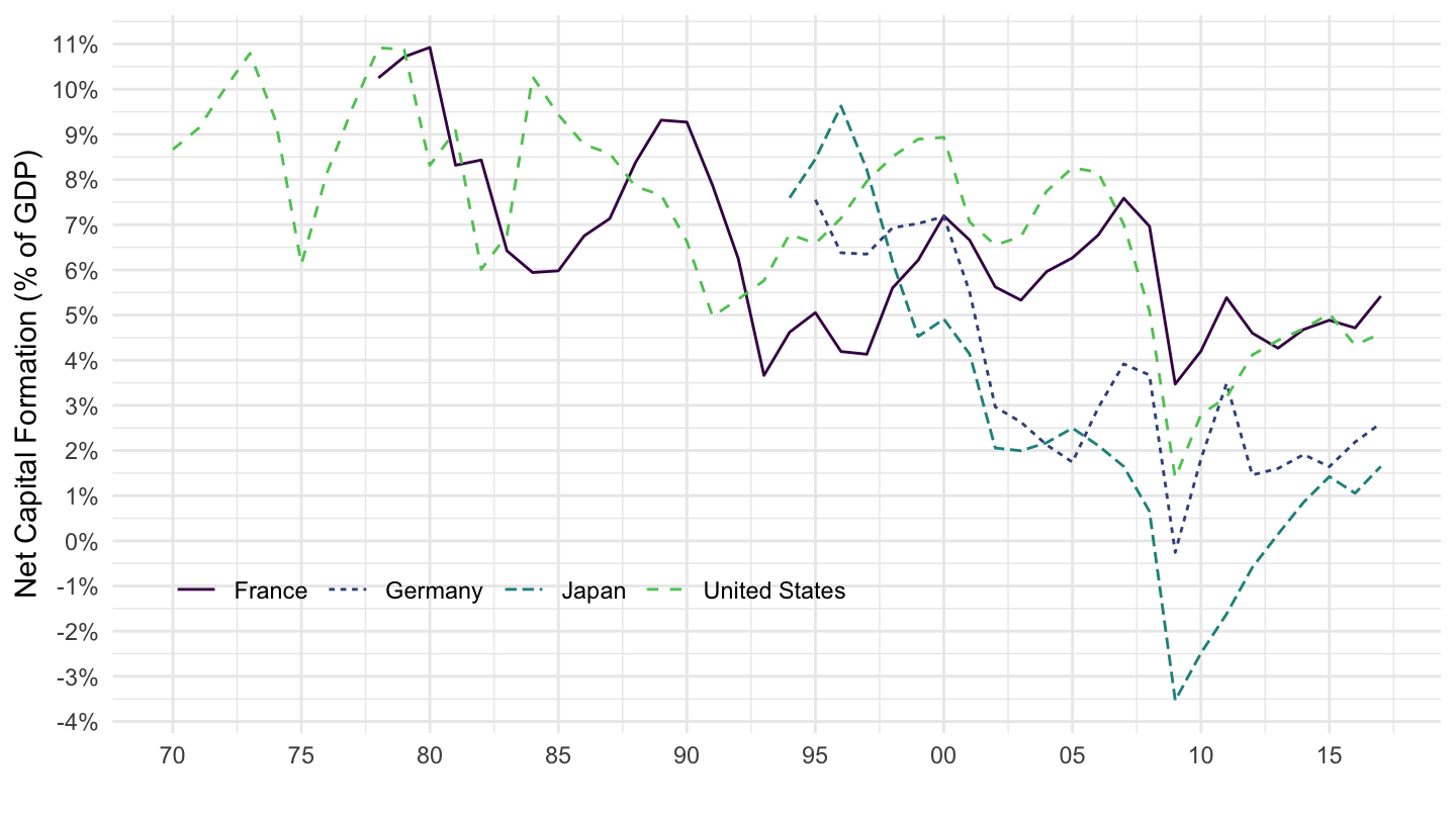

Ex 5: Operating surplus and mixed income; gross (% of GDP)

Code

SNA_TABLE14A_ARCHIVE %>%
  # NFB2G_B3GP: Operating surplus and mixed income
  filter(TRANSACT %in% c("NFB2G_B3GP", "B1_GE"),
         # S1: Total economy
         SECTOR == "S1",
         LOCATION %in% c("FRA", "USA", "DEU", "JPN")) %>%
  left_join(SNA_TABLE14A_ARCHIVE_var$LOCATION, by = c("LOCATION" = "id")) %>%
  select(LOCATION_desc = label, TRANSACT, obsTime, obsValue) %>%
  spread(TRANSACT, obsValue) %>%
  na.omit %>%
  year_to_date %>%
  mutate(value = NFB2G_B3GP / B1_GE) %>%
  ggplot() + theme_minimal() +
  geom_line(aes(x = date, y = value, color = LOCATION_desc, linetype = LOCATION_desc)) +
  scale_color_manual(values = viridis(5)[1:4]) +
  scale_x_date(breaks = seq(1920, 2025, 5) %>% paste0("-01-01") %>% as.Date,
               labels = date_format("%y")) +
  theme(legend.position = c(0.3, 0.8),
        legend.title = element_blank()) +
  scale_y_continuous(breaks = 0.01*seq(-60, 60, 1),
                     labels = scales::percent_format(accuracy = 1)) +
  ylab("Operating surplus and mixed income (% of GDP)") + xlab("")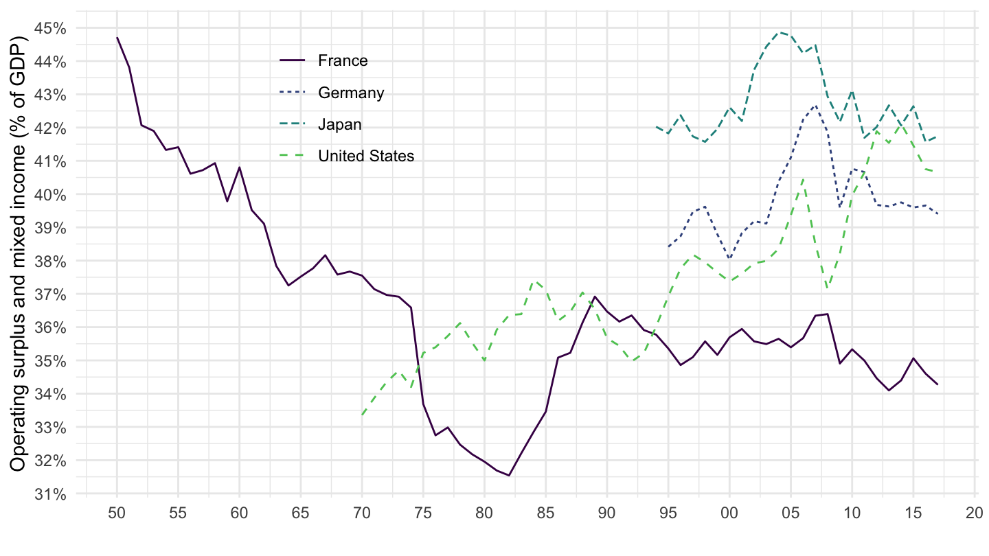

Ex 6: Adjustment for the change in net equity of households in pension funds -

Code

SNA_TABLE14A_ARCHIVE %>%
  # NFD8P: Adjustment for the change in net equity of households in pension funds 
  filter(TRANSACT %in% c("NFD8P", "B1_GE"),
         # S1: Total economy
         SECTOR == "S1",
         LOCATION %in% c("DEU", "DNK", "CAN", "JPN")) %>%
  left_join(SNA_TABLE14A_ARCHIVE_var$LOCATION, by = c("LOCATION" = "id")) %>%
  select(LOCATION_desc = label, TRANSACT, obsTime, obsValue) %>%
  spread(TRANSACT, obsValue) %>%
  na.omit %>%
  year_to_date %>%
  mutate(surplus_mixed_B1_GE = NFD8P / B1_GE) %>%
  ggplot() + theme_minimal() +
  geom_line(aes(x = date, y = surplus_mixed_B1_GE, color = LOCATION_desc, linetype = LOCATION_desc)) +
  scale_color_manual(values = viridis(5)[1:4]) +
  scale_x_date(breaks = seq(1920, 2025, 5) %>% paste0("-01-01") %>% as.Date,
               labels = date_format("%y")) +
  theme(legend.position = c(0.2, 0.2),
        legend.title = element_blank()) +
  scale_y_continuous(breaks = 0.01*seq(-60, 60, 1),
                     labels = scales::percent_format(accuracy = 1)) +
  ylab("Change in net equity of households in pension funds (% of GDP)") + xlab("")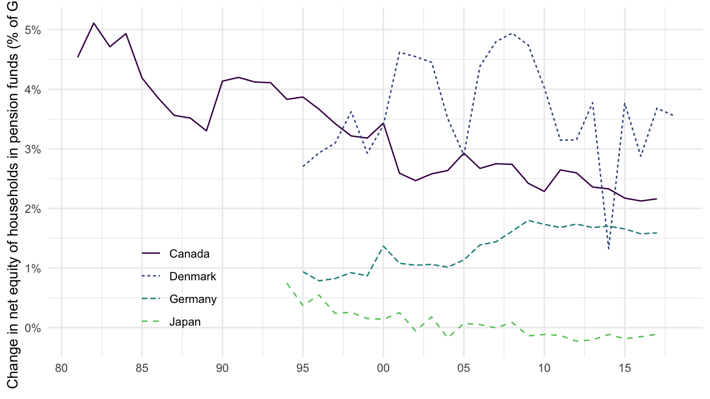

Ex 7: djustment for the change in net equity of households in pension funds (% of GDP)

Code

SNA_TABLE14A_ARCHIVE %>%
  # NFD8P: Adjustment for the change in net equity of households in pension funds 
  filter(TRANSACT %in% c("NFD8P", "B1_GE"), 
         SECTOR == "S1") %>%
  left_join(SNA_TABLE14A_ARCHIVE_var$LOCATION, by = c("LOCATION" = "id")) %>%
  select(Country = label, TRANSACT, obsTime, obsValue) %>%
  spread(TRANSACT, obsValue) %>%
  na.omit %>%
  mutate(NFD8P_B1_GE = (100*NFD8P / B1_GE)  %>% round(2) %>% paste("%")) %>%
  select(Country, obsTime, NFD8P_B1_GE) %>%
  group_by(Country) %>%
  summarise(year_first = first(obsTime),
            value_first = first(NFD8P_B1_GE),
            year_last = last(obsTime),
            value_last = last(NFD8P_B1_GE)) %>%
  {if (is_html_output()) datatable(., filter = 'top', rownames = F) else .}