Code
tibble(LAST_DOWNLOAD = as.Date(file.info("~/iCloud/website/data/oecd/SNA_TABLE12.RData")$mtime)) %>%
print_table_conditional()| LAST_DOWNLOAD |
|---|
| 2023-09-09 |
Data - OECD
tibble(LAST_DOWNLOAD = as.Date(file.info("~/iCloud/website/data/oecd/SNA_TABLE12.RData")$mtime)) %>%
print_table_conditional()| LAST_DOWNLOAD |
|---|
| 2023-09-09 |
| LAST_COMPILE |
|---|
| 2026-07-26 |
| obsTime | Nobs |
|---|---|
| 2022 | 8599 |
SNA_TABLE12 %>%
  left_join(SNA_TABLE12_var$TRANSACT %>%
              setNames(c("TRANSACT", "TRANSACT desc")), by = "TRANSACT") %>%
  left_join(SNA_TABLE12_var$SECTOR %>%
              setNames(c("SECTOR", "SECTOR desc")), by = "SECTOR") %>%
  group_by(TRANSACT, `TRANSACT desc`, SECTOR, `SECTOR desc`) %>%
  summarise(Nobs = n()) %>%
  arrange(-Nobs) %>%
{if (is_html_output()) datatable(., filter = 'top', rownames = F) else .}SNA_TABLE12_var$VAR_DESC %>%
{if (is_html_output()) print_table(.) else .}| id | description |
|---|---|
| LOCATION | Country |
| TRANSACT | Transaction |
| SECTOR | Sector |
| MEASURE | Measure |
| TIME | Year |
| OBS_VALUE | Observation Value |
| TIME_FORMAT | Time Format |
| OBS_STATUS | Observation Status |
| UNIT | Unit |
| POWERCODE | Unit multiplier |
| REFERENCEPERIOD | Reference period |
SNA_TABLE12 %>%
  left_join(SNA_TABLE12_var$TRANSACT %>%
              setNames(c("TRANSACT", "TRANSACT desc")), by = "TRANSACT") %>%
  group_by(TRANSACT, `TRANSACT desc`) %>%
  summarise(Nobs = n()) %>%
  arrange(-Nobs) %>%
{if (is_html_output()) datatable(., filter = 'top', rownames = F) else .}SNA_TABLE12 %>%
left_join(SNA_TABLE12_var$SECTOR %>%
setNames(c("SECTOR", "SECTOR desc")), by = "SECTOR") %>%
group_by(SECTOR, `SECTOR desc`) %>%
summarise(Nobs = n()) %>%
arrange(-Nobs) %>%
{if (is_html_output()) print_table(.) else .}| SECTOR | SECTOR desc | Nobs |
|---|---|---|
| GS13 | General government | 92437 |
| GS1311 | Central government | 91206 |
| GS1313 | Local government | 83895 |
| GS1314 | Social security funds | 73964 |
| GS1312 | State government | 27068 |
| S1 | Total economy | 2706 |
SNA_TABLE12 %>%
  filter(LOCATION %in% c("DEU", "FRA", "USA", "GBR"),
         # 020: Defense
         obsTime == "2017",
         # GS13: General government
         SECTOR == "GS13") %>%
  left_join(SNA_TABLE12_var$TRANSACT %>%
              setNames(c("TRANSACT", "TRANSACT desc")), by = "TRANSACT") %>%
  left_join(SNA_TABLE1 %>%
              filter(TRANSACT == "B1_GE",
                     MEASURE == "C") %>%
              select(obsTime, LOCATION, B1_GE = obsValue),
            by = c("LOCATION", "obsTime")) %>%
  mutate(obsValue = round(100*obsValue / B1_GE, 2) %>% paste0(" %")) %>%
  select(TRANSACT, `TRANSACT desc`, LOCATION, obsValue) %>%
  spread(LOCATION, obsValue) %>%
{if (is_html_output()) datatable(., filter = 'top', rownames = F) else .}SNA_TABLE12 %>%
filter(LOCATION %in% c("DEU", "FRA", "USA"),
TRANSACT == "GB9",
SECTOR == "GS13") %>%
left_join(SNA_TABLE12_var$LOCATION %>%
setNames(c("LOCATION", "LOCATION desc")), by = "LOCATION") %>%
left_join(SNA_TABLE1 %>%
filter(TRANSACT == "B1_GE",
MEASURE == "C") %>%
select(obsTime, LOCATION, B1_GE = obsValue),
by = c("LOCATION", "obsTime")) %>%
mutate(obsValue = obsValue / B1_GE) %>%
year_to_enddate %>%
ggplot() + theme_minimal() + ylab("Government Surplus (% of GDP)") + xlab("") +
geom_line(aes(x = date, y = obsValue, color = `LOCATION desc`, linetype = `LOCATION desc`)) +
scale_color_manual(values = viridis(4)[1:3]) +
scale_x_date(breaks = seq(1920, 2100, 5) %>% paste0("-01-01") %>% as.Date,
labels = date_format("%Y")) +
theme(legend.position = c(0.3, 0.2),
legend.title = element_blank(),
legend.direction = "horizontal") +
scale_y_continuous(breaks = 0.01*seq(-60, 60, 1),
labels = scales::percent_format(accuracy = 1))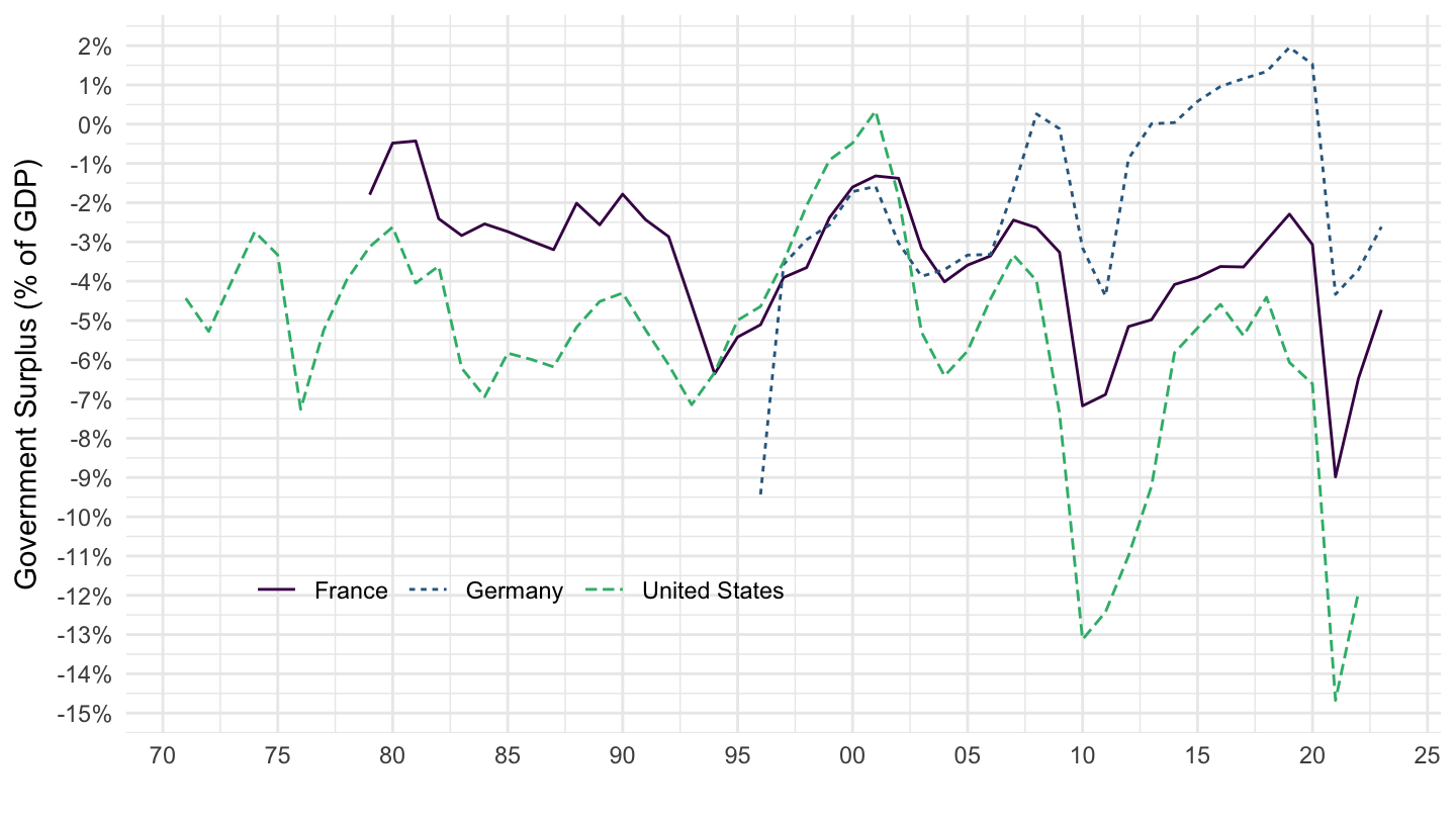
SNA_TABLE12 %>%
  filter(LOCATION %in% c("GBR", "FRA", "ESP"),
         TRANSACT == "GB9",
         SECTOR == "GS13") %>%
  left_join(SNA_TABLE12_var$LOCATION %>%
              setNames(c("LOCATION", "LOCATION desc")), by = "LOCATION") %>%
  left_join(SNA_TABLE1 %>%
              filter(TRANSACT == "B1_GE",
                     MEASURE == "C") %>%
              select(obsTime, LOCATION, B1_GE = obsValue),
            by = c("LOCATION", "obsTime")) %>%
  mutate(obsValue = obsValue / B1_GE) %>%
  year_to_enddate %>%
  ggplot() + theme_minimal() + ylab("Government Surplus (% of GDP)") + xlab("") +
  geom_line(aes(x = date, y = obsValue, color = `LOCATION desc`, linetype = `LOCATION desc`)) +
  scale_color_manual(values = viridis(4)[1:3]) +
  scale_x_date(breaks = seq(1920, 2100, 5) %>% paste0("-01-01") %>% as.Date,
               labels = date_format("%Y")) +
  theme(legend.position = c(0.3, 0.2),
        legend.title = element_blank(),
        legend.direction = "horizontal") +
  scale_y_continuous(breaks = 0.01*seq(-60, 60, 1),
                     labels = scales::percent_format(accuracy = 1))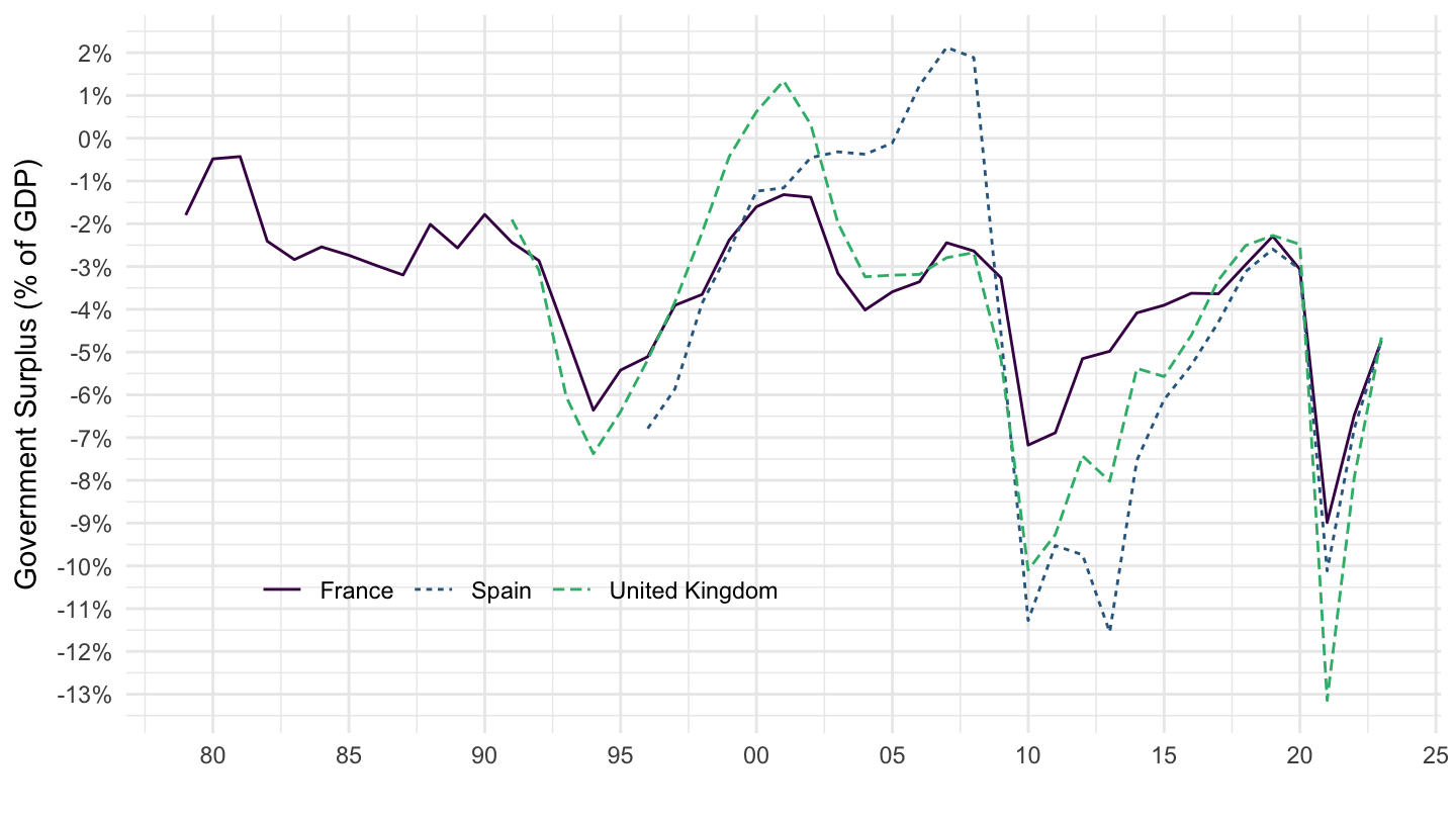
SNA_TABLE12 %>%
  filter(LOCATION %in% c("DEU", "FRA", "USA"),
         TRANSACT == "GP1R",
         SECTOR == "GS13") %>%
  left_join(SNA_TABLE12_var$LOCATION %>%
              setNames(c("LOCATION", "LOCATION desc")), by = "LOCATION") %>%
  left_join(SNA_TABLE1 %>%
              filter(TRANSACT == "B1_GE",
                     MEASURE == "C") %>%
              select(obsTime, LOCATION, B1_GE = obsValue),
            by = c("LOCATION", "obsTime")) %>%
  mutate(obsValue = obsValue / B1_GE) %>%
  year_to_enddate %>%
  ggplot() + theme_minimal() + ylab("Output (% of GDP)") + xlab("") +
  geom_line(aes(x = date, y = obsValue, color = `LOCATION desc`, linetype = `LOCATION desc`)) +
  scale_color_manual(values = viridis(4)[1:3]) +
  scale_x_date(breaks = seq(1920, 2100, 5) %>% paste0("-01-01") %>% as.Date,
               labels = date_format("%Y")) +
  theme(legend.position = c(0.3, 0.2),
        legend.title = element_blank(),
        legend.direction = "horizontal") +
  scale_y_continuous(breaks = 0.01*seq(-60, 60, 1),
                     labels = scales::percent_format(accuracy = 1))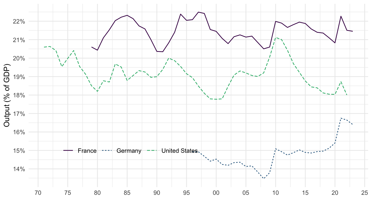
SNA_TABLE12 %>%
  filter(LOCATION %in% c("GBR", "FRA", "ESP"),
         TRANSACT == "GP1R",
         SECTOR == "GS13") %>%
  left_join(SNA_TABLE12_var$LOCATION %>%
              setNames(c("LOCATION", "LOCATION desc")), by = "LOCATION") %>%
  left_join(SNA_TABLE1 %>%
              filter(TRANSACT == "B1_GE",
                     MEASURE == "C") %>%
              select(obsTime, LOCATION, B1_GE = obsValue),
            by = c("LOCATION", "obsTime")) %>%
  mutate(obsValue = obsValue / B1_GE) %>%
  year_to_enddate %>%
  ggplot() + theme_minimal() + ylab("Output (% of GDP)") + xlab("") +
  geom_line(aes(x = date, y = obsValue, color = `LOCATION desc`, linetype = `LOCATION desc`)) +
  scale_color_manual(values = viridis(4)[1:3]) +
  scale_x_date(breaks = seq(1920, 2100, 5) %>% paste0("-01-01") %>% as.Date,
               labels = date_format("%Y")) +
  theme(legend.position = c(0.2, 0.2),
        legend.title = element_blank()) +
  scale_y_continuous(breaks = 0.01*seq(-60, 60, 1),
                     labels = scales::percent_format(accuracy = 1))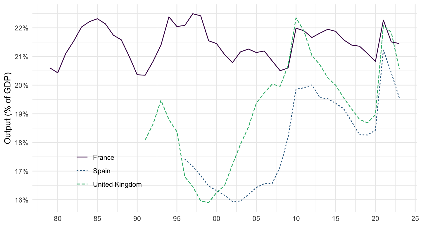
SNA_TABLE12 %>%
  filter(LOCATION %in% c("DEU", "FRA", "USA"),
         TRANSACT == "GD62_631XXP",
         SECTOR == "GS13") %>%
  left_join(SNA_TABLE12_var$LOCATION %>%
              setNames(c("LOCATION", "LOCATION desc")), by = "LOCATION") %>%
  left_join(SNA_TABLE1 %>%
              filter(TRANSACT == "B1_GE",
                     MEASURE == "C") %>%
              select(obsTime, LOCATION, B1_GE = obsValue),
            by = c("LOCATION", "obsTime")) %>%
  mutate(obsValue = obsValue / B1_GE) %>%
  year_to_enddate %>%
  ggplot() + theme_minimal() + ylab("Social benefits and transfers in kind (% of GDP)") + xlab("") +
  geom_line(aes(x = date, y = obsValue, color = `LOCATION desc`, linetype = `LOCATION desc`)) +
  scale_color_manual(values = viridis(4)[1:3]) +
  scale_x_date(breaks = seq(1920, 2100, 5) %>% paste0("-01-01") %>% as.Date,
               labels = date_format("%Y")) +
  theme(legend.position = c(0.2, 0.9),
        legend.title = element_blank()) +
  scale_y_continuous(breaks = 0.01*seq(-60, 60, 1),
                     labels = scales::percent_format(accuracy = 1))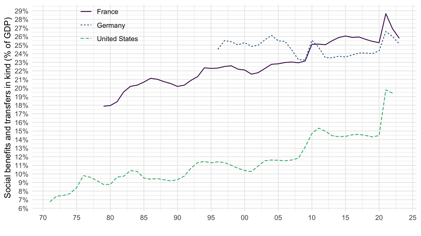
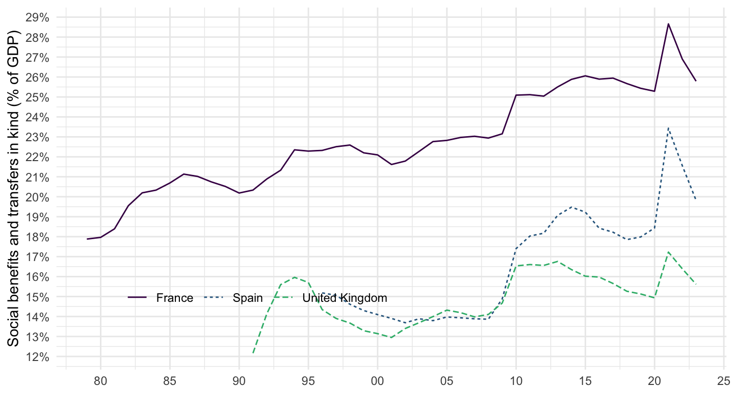
SNA_TABLE12 %>%
  filter(LOCATION %in% c("GBR", "FRA", "ESP"),
         TRANSACT == "GD62_631XXP",
         SECTOR == "GS13") %>%
  left_join(SNA_TABLE12_var$LOCATION %>%
              setNames(c("LOCATION", "LOCATION desc")), by = "LOCATION") %>%
  left_join(SNA_TABLE1 %>%
              filter(TRANSACT == "B1_GE",
                     MEASURE == "C") %>%
              select(obsTime, LOCATION, B1_GE = obsValue),
            by = c("LOCATION", "obsTime")) %>%
  mutate(obsValue = obsValue / B1_GE) %>%
  year_to_enddate %>%
  ggplot() + theme_minimal() + ylab("Social benefits and transfers in kind (% of GDP)") + xlab("") +
  geom_line(aes(x = date, y = obsValue, color = `LOCATION desc`, linetype = `LOCATION desc`)) +
  scale_color_manual(values = viridis(4)[1:3]) +
  scale_x_date(breaks = seq(1920, 2100, 5) %>% paste0("-01-01") %>% as.Date,
               labels = date_format("%Y")) +
  theme(legend.position = c(0.3, 0.2),
        legend.title = element_blank(),
        legend.direction = "horizontal") +
  scale_y_continuous(breaks = 0.01*seq(-60, 60, 1),
                     labels = scales::percent_format(accuracy = 1))