
Last observation: 2021 (N = 29214)
First observation: 1960 (N = 9)
Last data update: 02 août 2026, 09:09
Last compile: 07 oct. 2026, 23:51
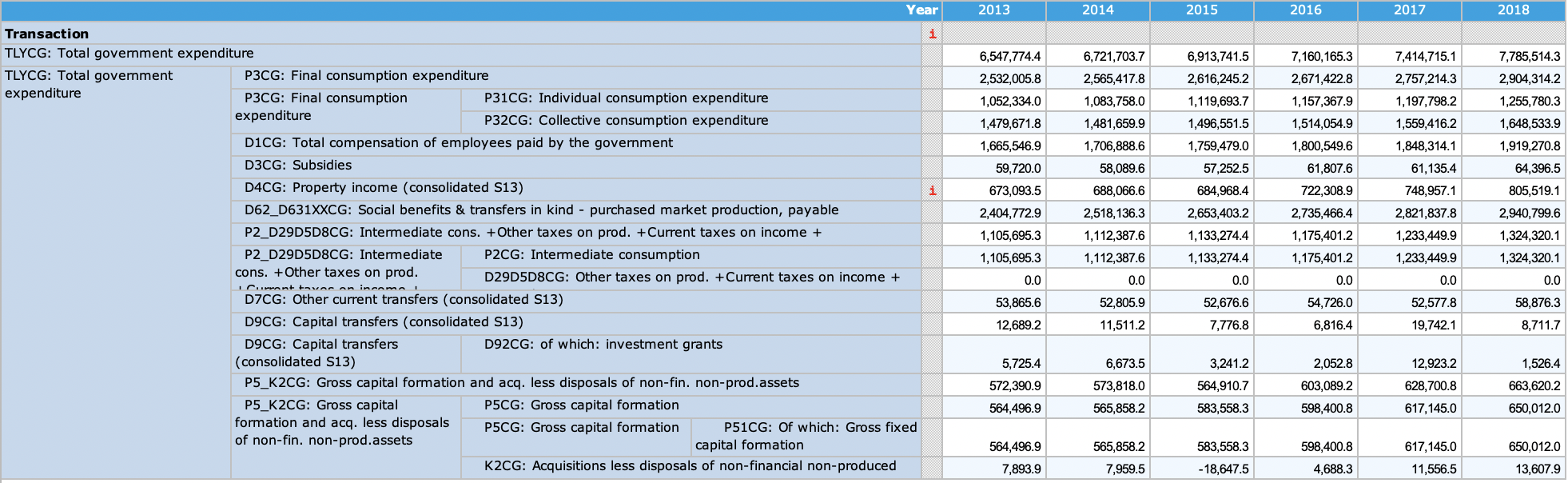
SNA_TABLE11 |>
  filter(LOCATION %in% c("DEU", "FRA", "USA", "GBR"),
         # TLYCG: Total government expenditure
         TRANSACT == "TLYCG",
         # 020: Defense
         obsTime == "2017",
         # GS13: General government
         SECTOR == "GS13") |>
  left_join(SNA_TABLE11_var$ACTIVITY, by = "ACTIVITY") |>
  left_join(SNA_TABLE1 |>
              filter(TRANSACT == "B1_GE",
                     MEASURE == "C") |>
              select(obsTime, LOCATION, B1_GE = obsValue),
            by = c("LOCATION", "obsTime")) |>
  mutate(obsValue = round(100*obsValue / B1_GE, 2) |> paste0(" %")) |>
  select(ACTIVITY, Activity, LOCATION, obsValue) |>
  spread(LOCATION, obsValue) |>
print_table_conditional()| ACTIVITY | Activity |
|---|---|
| character(0) | c(":--------:", ":--------:") |
SNA_TABLE11 |>
  filter(LOCATION == "DEU",
         # TLYCG: Total government expenditure
         TRANSACT == "TLYCG",
         # 070: Health; 090: Education; 100: Social protection
         ACTIVITY %in% c("070", "090", "100"),
         # GS13: General government
         SECTOR == "GS13") |>
  left_join(SNA_TABLE11_var$ACTIVITY, by = "ACTIVITY") |>
  year_to_enddate() |>
  ggplot() +
  geom_line(aes(x = date, y = obsValue/1000, color = Activity, linetype = Activity)) +
  theme_minimal()  +
  scale_color_manual(values = viridis(4)[1:3]) +
  scale_x_date(breaks = as.Date(paste0(seq(1960, 2020, 1), "-01-01")),
               labels = date_format("%Y")) +
  theme(legend.position = c(0.45, 0.9),
        legend.title = element_blank()) +
  xlab("") + ylab("") +
  scale_y_continuous(breaks = seq(0, 4000, 100),
                     labels = dollar_format(suffix = " Bn€", prefix = "", accuracy = 1))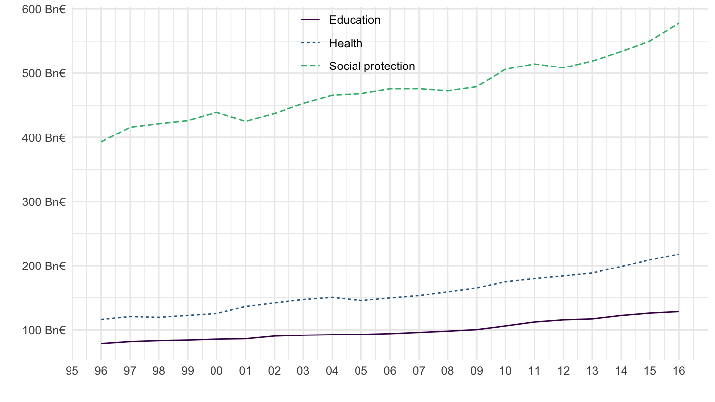
SNA_TABLE11 |>
  filter(LOCATION == "DEU",
         # TLYCG: Total government expenditure
         TRANSACT == "TLYCG",
         # 070: Health; 090: Education; 100: Social protection
         ACTIVITY %in% c("0701", "0702", "0703"),
         # GS13: General government
         SECTOR == "GS13") |>
  left_join(SNA_TABLE11_var$ACTIVITY, by = "ACTIVITY") |>
  year_to_enddate() |>
  ggplot() +
  geom_line(aes(x = date, y = obsValue/1000, color = Activity, linetype = Activity)) +
  theme_minimal()  +
  scale_color_manual(values = viridis(4)[1:3]) +
  scale_x_date(breaks = as.Date(paste0(seq(1960, 2020, 1), "-01-01")),
               labels = date_format("%Y")) +
  theme(legend.position = c(0.25, 0.8),
        legend.title = element_blank()) +
  xlab("") + ylab("") +
  scale_y_log10(breaks = seq(0, 4000, 10),
                labels = dollar_format(suffix = " Bn€", prefix = "", accuracy = 1))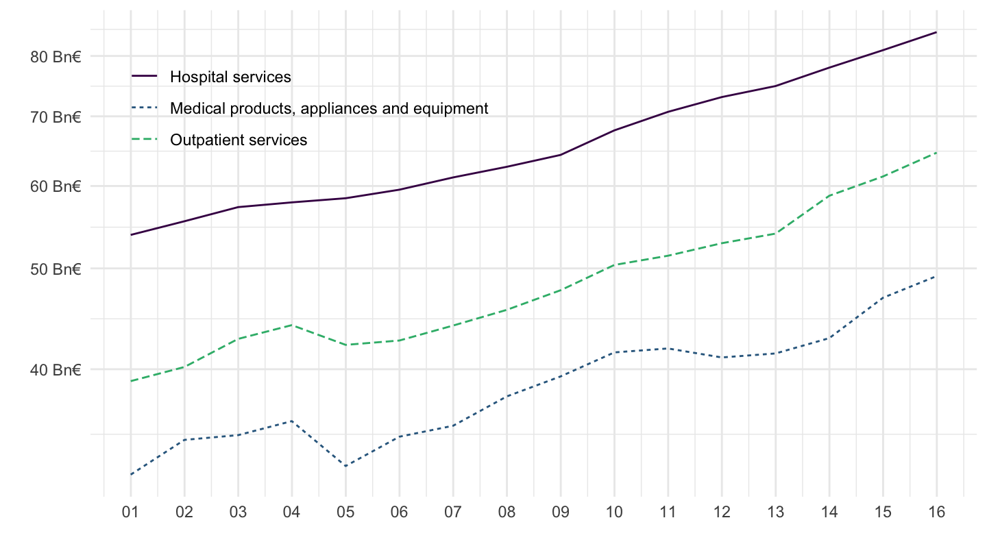
SNA_TABLE11 |>
  filter(LOCATION == "FRA",
         # TLYCG: Total government expenditure
         TRANSACT == "TLYCG",
         # 070: Health; 090: Education; 100: Social protection
         ACTIVITY %in% c("070", "090", "100"),
         # GS13: General government
         SECTOR == "GS13") |>
  left_join(SNA_TABLE11_var$ACTIVITY, by = "ACTIVITY") |>
  year_to_enddate() |>
  ggplot() +
  geom_line(aes(x = date, y = obsValue/1000, color = Activity, linetype = Activity)) +
  theme_minimal()  +
  scale_color_manual(values = viridis(4)[1:3]) +
  scale_x_date(breaks = as.Date(paste0(seq(1960, 2020, 1), "-01-01")),
               labels = date_format("%Y")) +
  theme(legend.position = c(0.15, 0.9),
        legend.title = element_blank()) +
  xlab("") + ylab("") +
  scale_y_log10(breaks = seq(0, 4000, 100),
                     labels = dollar_format(suffix = " Bn€", prefix = "", accuracy = 1))
SNA_TABLE11 |>
  filter(LOCATION == "FRA",
         # TLYCG: Total government expenditure
         TRANSACT == "TLYCG",
         # 070: Health; 090: Education; 100: Social protection
         ACTIVITY %in% c("0701", "0702", "0703"),
         # GS13: General government
         SECTOR == "GS13") |>
  left_join(SNA_TABLE11_var$ACTIVITY, by = "ACTIVITY") |>
  year_to_enddate() |>
  ggplot() +
  geom_line(aes(x = date, y = obsValue/1000, color = Activity, linetype = Activity)) +
  theme_minimal()  +
  scale_color_manual(values = viridis(4)[1:3]) +
  scale_x_date(breaks = as.Date(paste0(seq(1960, 2020, 1), "-01-01")),
               labels = date_format("%Y")) +
  theme(legend.position = c(0.75, 0.2),
        legend.title = element_blank()) +
  xlab("") + ylab("") +
  scale_y_log10(breaks = seq(0, 4000, 10),
                labels = dollar_format(suffix = " Bn€", prefix = "", accuracy = 1))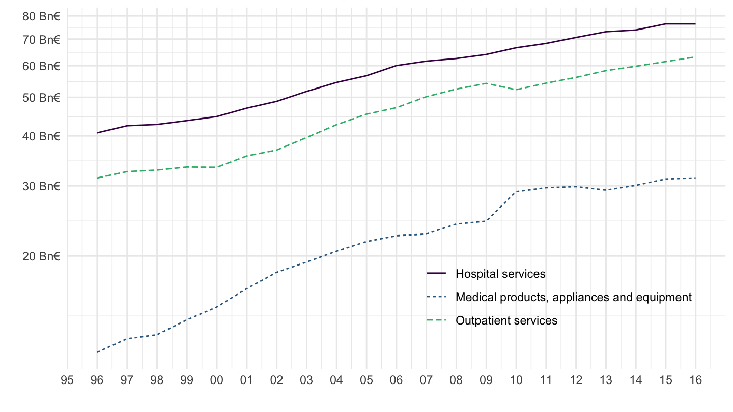
SNA_TABLE11 |>
  filter(LOCATION %in% c("DEU", "FRA", "ITA"),
         # TLYCG: Total government expenditure
         TRANSACT == "TLYCG",
         # 070: Health
         ACTIVITY %in% c("070"),
         # GS13: General government
         SECTOR == "GS13") |>
  left_join(SNA_TABLE11_var$LOCATION, by = "LOCATION") |>
  year_to_date() |>
  ggplot() + theme_minimal() + xlab("") + ylab("") +
  geom_line(aes(x = date, y = obsValue/1000, color = Location)) +
  geom_image(data = . %>%
               filter(date == as.Date("2015-01-01")) %>%
               mutate(image = paste0("../../icon/flag/", str_to_lower(Location), ".png")),
             aes(x = date, y = obsValue/1000, image = image), asp = 1.5) +
  scale_color_manual(values = c("#002395", "#000000", "#009246")) +
  scale_x_date(breaks = as.Date(paste0(seq(1960, 2020, 1), "-01-01")),
               labels = date_format("%Y")) +
  theme(legend.position = c(0.75, 0.2),
        legend.title = element_blank()) +
  scale_y_continuous(breaks = seq(0, 4000, 20),
                     labels = dollar_format(suffix = " Bn€", prefix = "", accuracy = 1))
SNA_TABLE11 |>
  filter(LOCATION %in% c("DEU", "FRA", "ITA"),
         # TLYCG: Total government expenditure
         TRANSACT == "TLYCG",
         # 070: Health
         ACTIVITY %in% c("070"),
         # GS13: General government
         SECTOR == "GS13") |>
  left_join(SNA_TABLE11_var$LOCATION, by = "LOCATION") |>
  year_to_date() |>
  ggplot() + theme_minimal() + xlab("") + ylab("") +
  geom_line(aes(x = date, y = obsValue/1000, color = Location)) +
  geom_image(data = . %>%
               filter(date == as.Date("2015-01-01")) %>%
               mutate(image = paste0("../../icon/flag/", str_to_lower(Location), ".png")),
             aes(x = date, y = obsValue/1000, image = image), asp = 1.5) +
  scale_color_manual(values = c("#002395", "#000000", "#009246")) +
  scale_x_date(breaks = as.Date(paste0(seq(1960, 2020, 1), "-01-01")),
               labels = date_format("%Y")) +
  theme(legend.position = c(0.75, 0.2),
        legend.title = element_blank()) +
  scale_y_log10(breaks = seq(0, 4000, 20),
                     labels = dollar_format(suffix = " Bn€", prefix = "", accuracy = 1))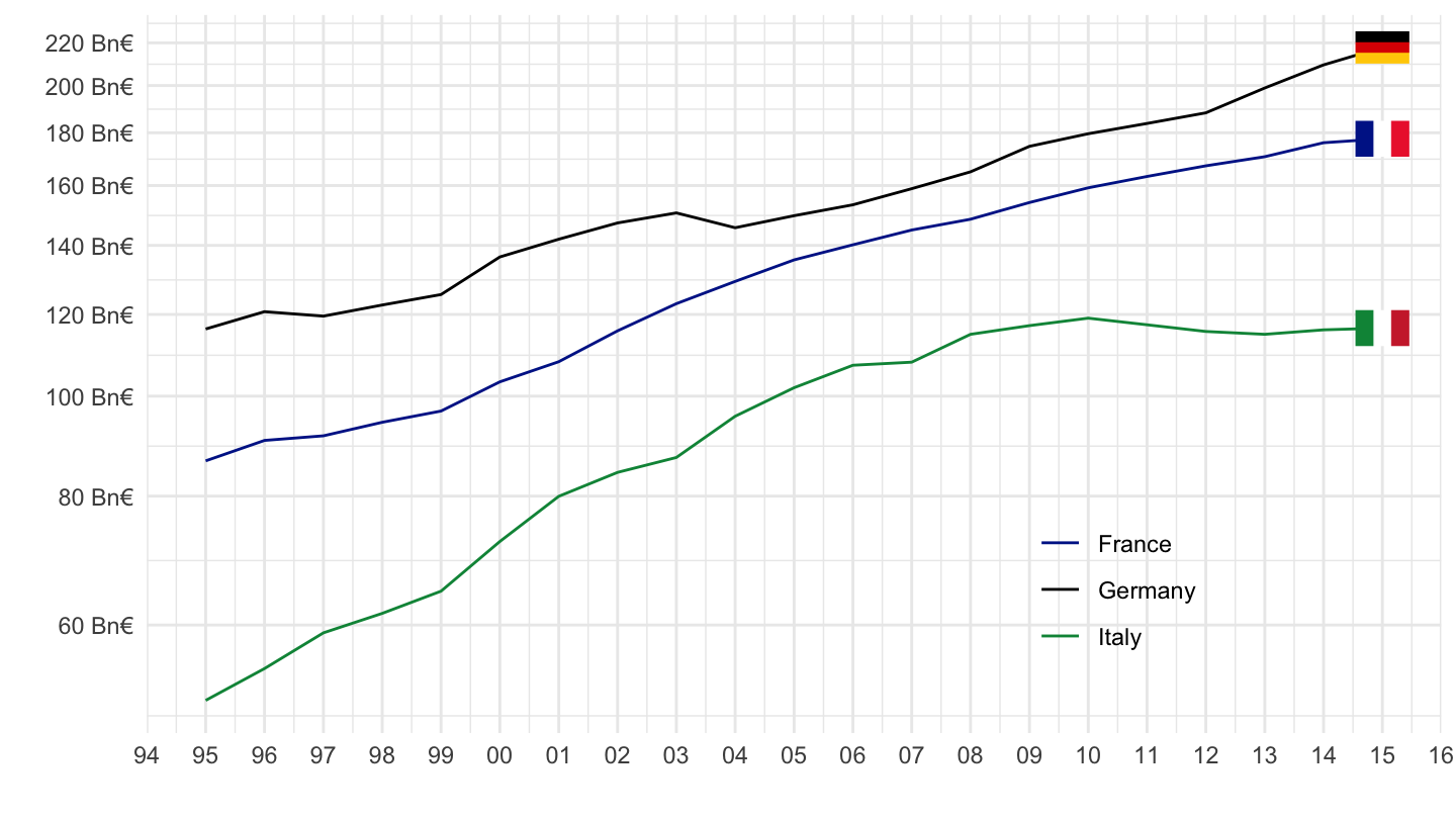
SNA_TABLE11 |>
  filter(LOCATION %in% c("DEU", "FRA", "ITA"),
         # TLYCG: Total government expenditure
         TRANSACT == "TLYCG",
         # 070: Health
         ACTIVITY %in% c("070"),
         # GS13: General government
         SECTOR == "GS13") |>
  left_join(SNA_TABLE11_var$LOCATION, by = "LOCATION") |>
  left_join(SNA_TABLE1 |>
              filter(TRANSACT == "B1_GE",
                     MEASURE == "C") |>
              select(obsTime, LOCATION, B1_GE = obsValue),
            by = c("LOCATION", "obsTime")) |>
  mutate(obsValue = obsValue / B1_GE) |>
  year_to_date() |>
  ggplot() + theme_minimal() + xlab("") + ylab("Health (% of GDP)") +
  geom_line(aes(x = date, y = obsValue, color = Location)) +
  scale_color_manual(values = c("#002395", "#000000", "#009246")) +
  geom_image(data = . %>%
               filter(date == as.Date("1995-01-01")) %>%
               mutate(image = paste0("../../icon/flag/", str_to_lower(Location), ".png")),
             aes(x = date, y = obsValue, image = image), asp = 1.5) +
  scale_x_date(breaks = as.Date(paste0(seq(1960, 2020, 1), "-01-01")),
               labels = date_format("%Y")) +
  scale_y_continuous(breaks = 0.01*seq(-60, 60, 1),
                     labels = scales::percent_format(accuracy = 1),
                     limits = c(0, 0.085)) +
  theme(legend.position = c(0.85, 0.2),
        legend.title = element_blank())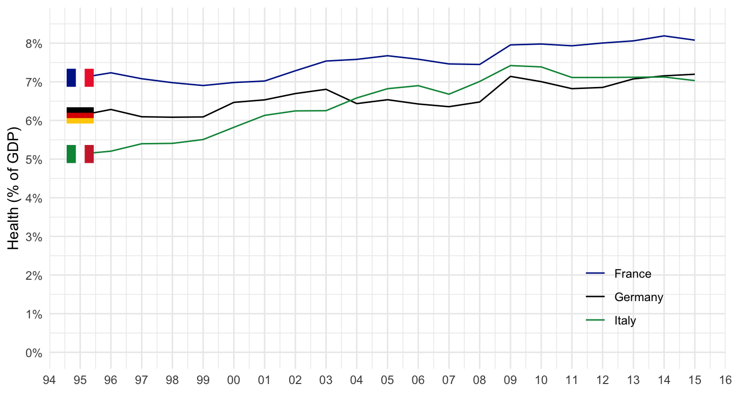
SNA_TABLE11 |>
  filter(LOCATION %in% c("DEU", "FRA", "ITA"),
         # TLYCG: Total government expenditure
         TRANSACT == "TLYCG",
         # 070: Health
         ACTIVITY %in% c("070"),
         # GS13: General government
         SECTOR == "GS13") |>
  left_join(SNA_TABLE11_var$LOCATION, by = "LOCATION") |>
  left_join(SNA_TABLE1 |>
              filter(TRANSACT == "B1_GE",
                     MEASURE == "C") |>
              select(obsTime, LOCATION, B1_GE = obsValue),
            by = c("LOCATION", "obsTime")) |>
  group_by(LOCATION) |>
  mutate(B1_GE_t = log(B1_GE) |> hpfilter(100000) |> pluck("trend") |> exp(),
         obsValue = obsValue / B1_GE_t) |>
  year_to_date() |>
  ggplot() + theme_minimal() + xlab("") + ylab("Health (% of detrended GDP)") +
  geom_line(aes(x = date, y = obsValue, color = Location)) +
  geom_image(data = . %>%
               filter(date == as.Date("2015-01-01")) %>%
               mutate(image = paste0("../../icon/flag/", str_to_lower(Location), ".png")),
             aes(x = date, y = obsValue, image = image), asp = 1.5) +
  scale_color_manual(values = c("#002395", "#000000", "#009246")) +
  scale_x_date(breaks = as.Date(paste0(seq(1960, 2020, 1), "-01-01")),
               labels = date_format("%Y")) +
  scale_y_continuous(breaks = 0.01*seq(-60, 60, 1),
                     labels = scales::percent_format(accuracy = 1),
                     limits = c(0, 0.085)) +
  theme(legend.position = c(0.85, 0.2),
        legend.title = element_blank())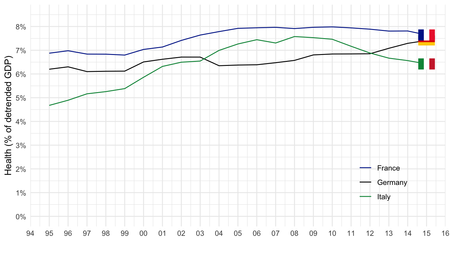
SNA_TABLE11 |>
  filter(LOCATION %in% c("DEU", "FRA", "ITA"),
         # TLYCG: Total government expenditure
         TRANSACT == "TLYCG",
         # 070: Health
         ACTIVITY %in% c("070"),
         # GS13: General government
         SECTOR == "GS13") |>
  left_join(SNA_TABLE11_var$LOCATION, by = "LOCATION") |>
  left_join(SNA_TABLE1 |>
              filter(TRANSACT == "B1_GE",
                     MEASURE == "C") |>
              select(obsTime, LOCATION, B1_GE = obsValue),
            by = c("LOCATION", "obsTime")) |>
  group_by(LOCATION) |>
  mutate(B1_GE_t = log(B1_GE) |> hpfilter(100000) |> pluck("trend") |> exp(),
         obsValue = obsValue / B1_GE_t) |>
  year_to_date() |>
  ggplot() + theme_minimal() + xlab("") + ylab("Health (% of detrended GDP)") +
  geom_line(aes(x = date, y = B1_GE/B1_GE_t, color = Location)) +
  geom_image(data = . %>%
               filter(date == as.Date("2018-01-01")) %>%
               mutate(image = paste0("../../icon/flag/", str_to_lower(Location), ".png")),
             aes(x = date, y = B1_GE/B1_GE_t, image = image), asp = 1.5) +
  scale_color_manual(values = c("#002395", "#000000", "#009246")) +
  scale_x_date(breaks = as.Date(paste0(seq(1960, 2020, 1), "-01-01")),
               labels = date_format("%Y")) +
  scale_y_continuous(breaks = 0.01*seq(-60, 150, 1),
                     labels = scales::percent_format(accuracy = 1)) +
  theme(legend.position = c(0.15, 0.85),
        legend.title = element_blank())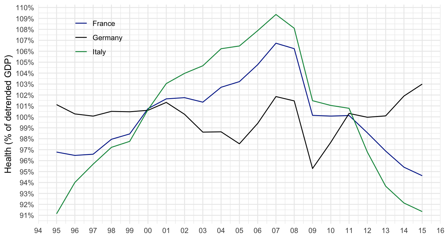
SNA_TABLE11 |>
  filter(LOCATION %in% c("DEU", "FRA", "ITA"),
         # TLYCG: Total government expenditure
         TRANSACT == "TLYCG",
         # 0701: Health
         ACTIVITY %in% c("0701"),
         # GS13: General government
         SECTOR == "GS13") |>
  left_join(SNA_TABLE11_var$LOCATION, by = "LOCATION") |>
  year_to_date() |>
  ggplot() + theme_minimal() + xlab("") + ylab("Medical products, appliances and equipment") +
  geom_line(aes(x = date, y = obsValue/1000, color = Location)) +
     scale_color_manual(values = c("#002395", "#000000", "#009246")) +
  geom_image(data = . %>%
               filter(date == as.Date("2015-01-01")) %>%
               mutate(image = paste0("../../icon/flag/", str_to_lower(Location), ".png")),
             aes(x = date, y = obsValue/1000, image = image), asp = 1.5) +
  scale_x_date(breaks = as.Date(paste0(seq(1960, 2020, 1), "-01-01")),
               labels = date_format("%Y")) +
  theme(legend.position = c(0.15, 0.8),
        legend.title = element_blank()) +
  scale_y_continuous(breaks = seq(0, 4000, 10),
                     labels = dollar_format(suffix = " Bn€", prefix = "", accuracy = 1))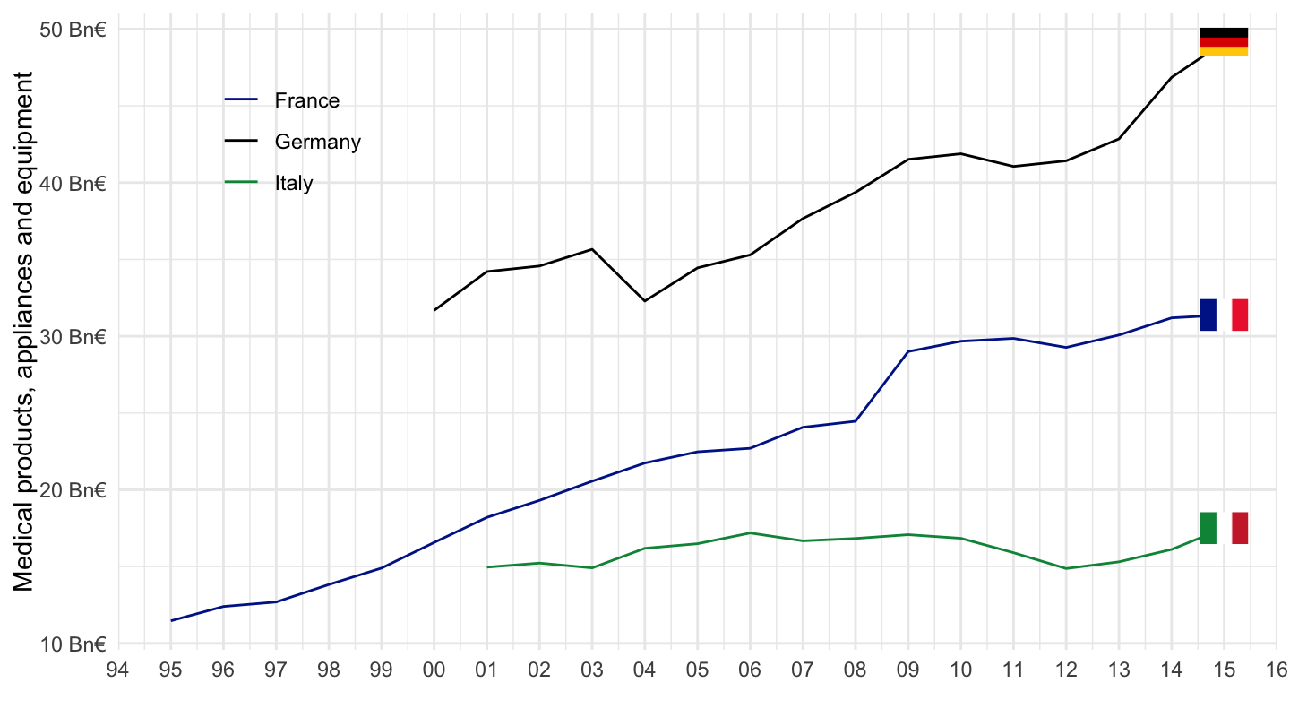
SNA_TABLE11 |>
  filter(LOCATION %in% c("DEU", "FRA", "ITA"),
         # TLYCG: Total government expenditure
         TRANSACT == "TLYCG",
         # 0701: Health
         ACTIVITY %in% c("0701"),
         # GS13: General government
         SECTOR == "GS13") |>
  left_join(SNA_TABLE11_var$LOCATION, by = "LOCATION") |>
  year_to_date() |>
  ggplot() + theme_minimal() + xlab("") + ylab("Medical products, appliances and equipment") +
  geom_line(aes(x = date, y = obsValue/1000, color = Location)) +
  scale_color_manual(values = c("#002395", "#000000", "#009246")) +
  geom_image(data = . %>%
               filter(date == as.Date("2015-01-01")) %>%
               mutate(image = paste0("../../icon/flag/", str_to_lower(Location), ".png")),
             aes(x = date, y = obsValue/1000, image = image), asp = 1.5) +
  scale_x_date(breaks = as.Date(paste0(seq(1960, 2020, 1), "-01-01")),
               labels = date_format("%Y")) +
  theme(legend.position = c(0.15, 0.8),
        legend.title = element_blank()) +
  scale_y_log10(breaks = seq(0, 4000, 5),
                     labels = dollar_format(suffix = " Bn€", prefix = "", accuracy = 1))
SNA_TABLE11 |>
  filter(LOCATION %in% c("DEU", "FRA", "ITA"),
         # TLYCG: Total government expenditure
         TRANSACT == "TLYCG",
         # 0701: Health
         ACTIVITY %in% c("0701"),
         # GS13: General government
         SECTOR == "GS13") |>
  left_join(SNA_TABLE11_var$LOCATION, by = "LOCATION") |>
  left_join(SNA_TABLE1 |>
              filter(TRANSACT == "B1_GE",
                     MEASURE == "C") |>
              select(obsTime, LOCATION, B1_GE = obsValue),
            by = c("LOCATION", "obsTime")) |>
  mutate(obsValue = obsValue / B1_GE) |>
  year_to_date() |>
  ggplot() + theme_minimal() + xlab("") + ylab("Medical products, appliances and equipment") +
  geom_line(aes(x = date, y = obsValue, color = Location)) +
  geom_image(data = . %>%
               filter(date == as.Date("2015-01-01")) %>%
               mutate(image = paste0("../../icon/flag/", str_to_lower(Location), ".png")),
             aes(x = date, y = obsValue, image = image), asp = 1.5) +
     scale_color_manual(values = c("#002395", "#000000", "#009246")) +
  scale_x_date(breaks = as.Date(paste0(seq(1960, 2020, 1), "-01-01")),
               labels = date_format("%Y")) +
  scale_y_continuous(breaks = 0.01*seq(-60, 60, 0.2),
                     labels = scales::percent_format(accuracy = 0.1),
                     limits = c(0, 0.018)) +
  theme(legend.position = c(0.85, 0.2),
        legend.title = element_blank())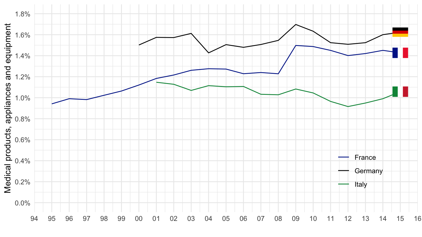
SNA_TABLE11 |>
  filter(LOCATION %in% c("DEU", "FRA", "ITA"),
         # TLYCG: Total government expenditure
         TRANSACT == "TLYCG",
         # 0701: Health
         ACTIVITY %in% c("0701"),
         # GS13: General government
         SECTOR == "GS13") |>
  left_join(SNA_TABLE11_var$LOCATION, by = "LOCATION") |>
  left_join(SNA_TABLE1 |>
              filter(TRANSACT == "B1_GE",
                     MEASURE == "C") |>
              select(obsTime, LOCATION, B1_GE = obsValue),
            by = c("LOCATION", "obsTime")) |>
  group_by(LOCATION) |>
  mutate(B1_GE_t = log(B1_GE) |> hpfilter(100000) |> pluck("trend") |> exp(),
         obsValue = obsValue / B1_GE_t) |>
  year_to_date() |>
  ggplot() + theme_minimal() + xlab("") + ylab("Medical products, appliances and equipment") +
  geom_line(aes(x = date, y = obsValue, color = Location)) +
  geom_image(data = . %>%
               filter(date == as.Date("2015-01-01")) %>%
               mutate(image = paste0("../../icon/flag/", str_to_lower(Location), ".png")),
             aes(x = date, y = obsValue, image = image), asp = 1.5) +
     scale_color_manual(values = c("#002395", "#000000", "#009246")) +
  scale_x_date(breaks = as.Date(paste0(seq(1960, 2020, 1), "-01-01")),
               labels = date_format("%Y")) +
  scale_y_continuous(breaks = 0.01*seq(-60, 60, 0.2),
                     labels = scales::percent_format(accuracy = 0.1),
                     limits = c(0, 0.018)) +
  theme(legend.position = c(0.85, 0.2),
        legend.title = element_blank())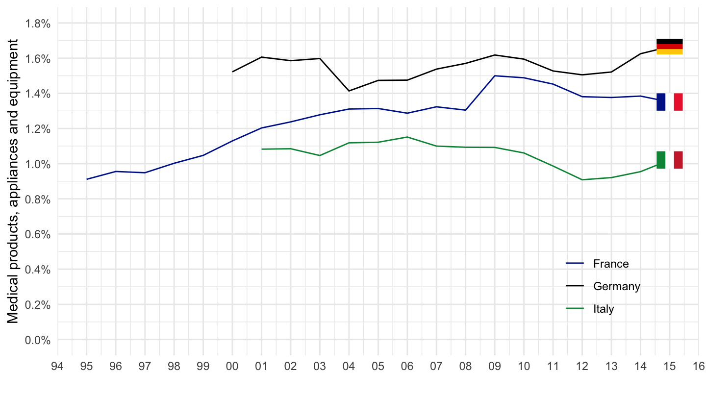
SNA_TABLE11 |>
  filter(LOCATION %in% c("DEU", "FRA", "ITA"),
         # TLYCG: Total government expenditure
         TRANSACT == "TLYCG",
         # 070: Health
         ACTIVITY %in% c("T"),
         # GS13: General government
         SECTOR == "GS13") |>
  left_join(SNA_TABLE11_var$LOCATION, by = "LOCATION") |>
  left_join(SNA_TABLE1 |>
              filter(TRANSACT == "B1_GE",
                     MEASURE == "C") |>
              select(obsTime, LOCATION, B1_GE = obsValue),
            by = c("LOCATION", "obsTime")) |>
  mutate(obsValue = obsValue / B1_GE) |>
  year_to_date() |>
  ggplot() + theme_minimal() + xlab("") + ylab("Total (% of GDP)") +
  geom_line(aes(x = date, y = obsValue, color = Location)) +
  geom_image(data = . %>%
               filter(date == as.Date("2015-01-01")) %>%
               mutate(image = paste0("../../icon/flag/", str_to_lower(Location), ".png")),
             aes(x = date, y = obsValue, image = image), asp = 1.5) +
     scale_color_manual(values = c("#002395", "#000000", "#009246")) +
  scale_x_date(breaks = as.Date(paste0(seq(1960, 2020, 1), "-01-01")),
               labels = date_format("%Y")) +
  scale_y_continuous(breaks = 0.01*seq(-60, 100, 5),
                     labels = scales::percent_format(accuracy = 1),
                     limits = c(0, 0.60)) +
  theme(legend.position = c(0.85, 0.2),
        legend.title = element_blank())
SNA_TABLE11 |>
  filter(LOCATION %in% c("USA", "FRA", "GBR"),
         # TLYCG: Total government expenditure
         TRANSACT == "TLYCG",
         # 070: Health
         ACTIVITY %in% c("T"),
         # GS13: General government
         SECTOR == "GS13") |>
  left_join(SNA_TABLE11_var$LOCATION, by = "LOCATION") |>
  left_join(SNA_TABLE1 |>
              filter(TRANSACT == "B1_GE",
                     MEASURE == "C") |>
              select(obsTime, LOCATION, B1_GE = obsValue),
            by = c("LOCATION", "obsTime")) |>
  mutate(obsValue = obsValue / B1_GE) |>
  year_to_date() |>
  filter(date >= as.Date("1994-12-01")) |>
  ggplot() + theme_minimal() + xlab("") + ylab("Total (% of GDP)") +
  geom_line(aes(x = date, y = obsValue, color = Location)) +
  geom_image(data = . %>%
               filter(date == as.Date("2015-01-01")) %>%
               mutate(image = paste0("../../icon/flag/", str_to_lower(gsub(" ", "-", Location)), ".png")),
             aes(x = date, y = obsValue, image = image), asp = 1.5) +
     scale_color_manual(values = c("#002395", "#CF142B", "#3C3B6E")) +
  scale_x_date(breaks = as.Date(paste0(seq(1960, 2020, 2), "-01-01")),
               labels = date_format("%Y")) +
  scale_y_continuous(breaks = 0.01*seq(-60, 100, 5),
                     labels = scales::percent_format(accuracy = 1),
                     limits = c(0, 0.60)) +
  theme(legend.position = c(0.85, 0.2),
        legend.title = element_blank())
SNA_TABLE11 |>
  filter(LOCATION %in% c("DEU", "FRA", "ITA"),
         # TLYCG: Total government expenditure
         TRANSACT == "TLYCG",
         # 070: Health
         ACTIVITY %in% c("T"),
         # GS13: General government
         SECTOR == "GS13") |>
  left_join(SNA_TABLE11_var$LOCATION, by = "LOCATION") |>
  left_join(SNA_TABLE1 |>
              filter(TRANSACT == "B1_GE",
                     MEASURE == "C") |>
              select(obsTime, LOCATION, B1_GE = obsValue),
            by = c("LOCATION", "obsTime")) |>
  group_by(LOCATION) |>
  mutate(B1_GE_t = log(B1_GE) |> hpfilter(100000) |> pluck("trend") |> exp(),
         obsValue = obsValue / B1_GE_t) |>
  year_to_date() |>
  ggplot() + theme_minimal() + xlab("") + ylab("Total (% of detrended GDP)") +
  geom_line(aes(x = date, y = obsValue, color = Location)) +
  geom_image(data = . %>%
               filter(date == as.Date("2015-01-01")) %>%
               mutate(image = paste0("../../icon/flag/", str_to_lower(Location), ".png")),
             aes(x = date, y = obsValue, image = image), asp = 1.5) +
     scale_color_manual(values = c("#002395", "#000000", "#009246")) +
  scale_x_date(breaks = as.Date(paste0(seq(1960, 2020, 1), "-01-01")),
               labels = date_format("%Y")) +
  scale_y_continuous(breaks = 0.01*seq(-60, 100, 5),
                     labels = scales::percent_format(accuracy = 1),
                     limits = c(0, 0.60)) +
  theme(legend.position = c(0.85, 0.2),
        legend.title = element_blank())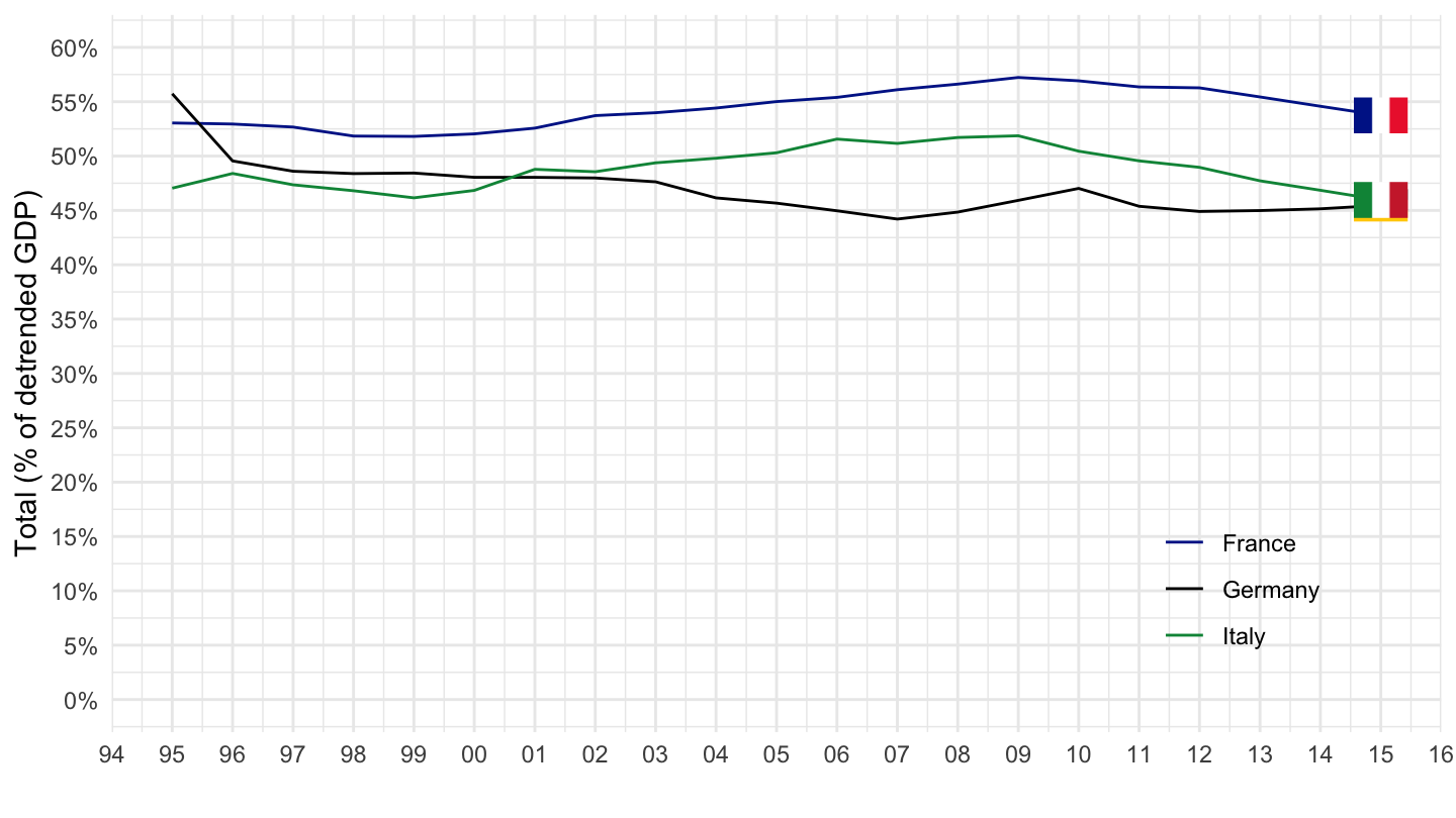
SNA_TABLE11 |>
  filter(LOCATION %in% c("DEU", "FRA", "ITA"),
         # TLYCG: Total government expenditure
         TRANSACT == "TLYCG",
         # 070: Health
         ACTIVITY %in% c("090"),
         # GS13: General government
         SECTOR == "GS13") |>
  left_join(SNA_TABLE11_var$LOCATION, by = "LOCATION") |>
  left_join(SNA_TABLE1 |>
              filter(TRANSACT == "B1_GE",
                     MEASURE == "C") |>
              select(obsTime, LOCATION, B1_GE = obsValue),
            by = c("LOCATION", "obsTime")) |>
  mutate(obsValue = obsValue / B1_GE) |>
  year_to_date() |>
  ggplot() + theme_minimal() + xlab("") + ylab("Education (% of GDP)") +
  geom_line(aes(x = date, y = obsValue, color = Location)) + add_3flags +
     scale_color_manual(values = c("#002395", "#000000", "#009246")) +
  scale_x_date(breaks = as.Date(paste0(seq(1960, 2020, 5), "-01-01")),
               labels = date_format("%Y")) +
  scale_y_continuous(breaks = 0.01*seq(-60, 60, .2),
                     labels = scales::percent_format(accuracy = .1)) +
  theme(legend.position = c(0.85, 0.2),
        legend.title = element_blank())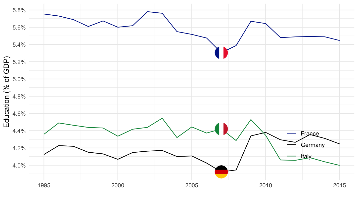
SNA_TABLE11 |>
  filter(LOCATION %in% c("DEU", "FRA", "ITA"),
         # TLYCG: Total government expenditure
         TRANSACT == "TLYCG",
         # 070: Health
         ACTIVITY %in% c("090"),
         # GS13: General government
         SECTOR == "GS13") |>
  left_join(SNA_TABLE11_var$LOCATION, by = "LOCATION") |>
  left_join(SNA_TABLE1 |>
              filter(TRANSACT == "B1_GE",
                     MEASURE == "C") |>
              select(obsTime, LOCATION, B1_GE = obsValue),
            by = c("LOCATION", "obsTime")) |>
  group_by(LOCATION) |>
  mutate(B1_GE_t = log(B1_GE) |> hpfilter(100000) |> pluck("trend") |> exp(),
         obsValue = obsValue / B1_GE_t) |>
  year_to_date() |>
  ggplot() + theme_minimal() + xlab("") + ylab("Education (% of detrended GDP)") +
  geom_line(aes(x = date, y = obsValue, color = Location)) +
  geom_image(data = . %>%
               filter(date == as.Date("2015-01-01")) %>%
               mutate(image = paste0("../../icon/flag/", str_to_lower(Location), ".png")),
             aes(x = date, y = obsValue, image = image), asp = 1.5) +
     scale_color_manual(values = c("#002395", "#000000", "#009246")) +
  scale_x_date(breaks = as.Date(paste0(seq(1960, 2020, 1), "-01-01")),
               labels = date_format("%Y")) +
  scale_y_continuous(breaks = 0.01*seq(-60, 60, 1),
                     labels = scales::percent_format(accuracy = 1),
                     limits = c(0, 0.06)) +
  theme(legend.position = c(0.85, 0.2),
        legend.title = element_blank())
SNA_TABLE11 |>
  filter(LOCATION %in% c("DEU", "FRA", "ITA", "USA", "RUS"),
         # TLYCG: Total government expenditure
         TRANSACT == "TLYCG",
         # 020: Defense
         ACTIVITY %in% c("020"),
         # GS13: General government
         SECTOR == "GS13") |>
  left_join(SNA_TABLE11_var$LOCATION, by = "LOCATION") |>
  left_join(SNA_TABLE1 |>
              filter(TRANSACT == "B1_GE",
                     MEASURE == "C") |>
              select(obsTime, LOCATION, B1_GE = obsValue),
            by = c("LOCATION", "obsTime")) |>
  mutate(obsValue = obsValue / B1_GE) |>
  year_to_date() |>
  filter(date >= as.Date("1995-01-01")) |>
  add_flag_color("Location") |>
  ggplot() + theme_minimal() + xlab("") + ylab("Defense (% of GDP)") +
  geom_line(aes(x = date, y = obsValue, color = color)) + add_4flags +
     scale_color_identity() +
  scale_x_date(breaks = as.Date(paste0(seq(1960, 2020, 5), "-01-01")),
               labels = date_format("%Y")) +
  scale_y_continuous(breaks = 0.01*seq(-60, 60, 0.5),
                     labels = scales::percent_format(accuracy = 0.1)) +
  theme(legend.position = c(0.85, 0.2),
        legend.title = element_blank())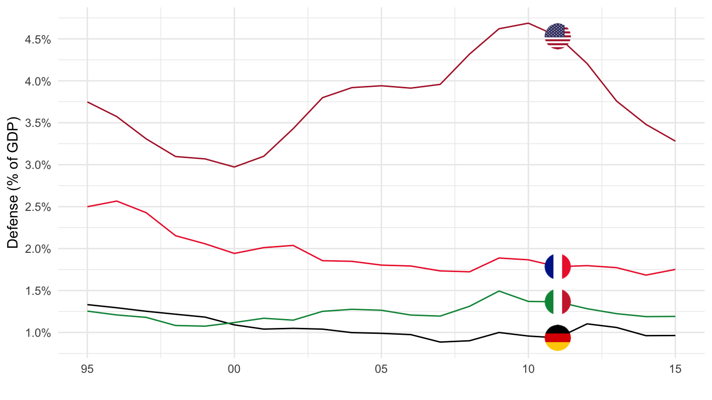
SNA_TABLE11 |>
  filter(LOCATION %in% c("DEU", "FRA", "ITA"),
         # TLYCG: Total government expenditure
         TRANSACT == "TLYCG",
         # 020: Defense
         ACTIVITY %in% c("020"),
         # GS13: General government
         SECTOR == "GS13") |>
  left_join(SNA_TABLE11_var$LOCATION, by = "LOCATION") |>
  left_join(SNA_TABLE1 |>
              filter(TRANSACT == "B1_GE",
                     MEASURE == "C") |>
              select(obsTime, LOCATION, B1_GE = obsValue),
            by = c("LOCATION", "obsTime")) |>
  group_by(LOCATION) |>
  mutate(B1_GE_t = log(B1_GE) |> hpfilter(100000) |> pluck("trend") |> exp(),
         obsValue = obsValue / B1_GE_t) |>
  year_to_date() |>
  ggplot() + theme_minimal() + xlab("") + ylab("Defense (% of detrended GDP)") +
  geom_line(aes(x = date, y = obsValue, color = Location)) +
  geom_image(data = . %>%
               filter(date == as.Date("2015-01-01")) %>%
               mutate(image = paste0("../../icon/flag/", str_to_lower(Location), ".png")),
             aes(x = date, y = obsValue, image = image), asp = 1.5) +
     scale_color_manual(values = c("#002395", "#000000", "#009246")) +
  scale_x_date(breaks = as.Date(paste0(seq(1960, 2020, 1), "-01-01")),
               labels = date_format("%Y")) +
  scale_y_continuous(breaks = 0.01*seq(-60, 60, 0.5),
                     labels = scales::percent_format(accuracy = 0.1),
                     limits = c(0, 0.027)) +
  theme(legend.position = c(0.85, 0.2),
        legend.title = element_blank())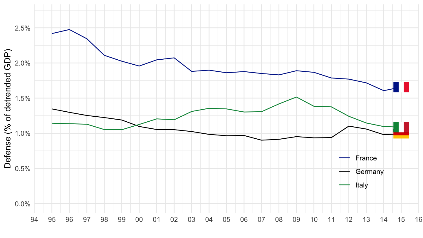
100 - Social protection
% of GDP
Code
% of GDP
Code
% of detrended GDP
Code