Taxes and social contributions receipts - SNA_TABLE10

Data - OECD

load_data("oecd/SNA_TABLE10_var.RData")
SNA_TABLE10 <- read_parquet("SNA_TABLE10.parquet")
load_data("oecd/SNA_TABLE1_var.RData")
SNA_TABLE1 <- read_parquet("SNA_TABLE1.parquet")

Last observation: 2022 (N = 2207)

First observation: 1950 (N = 4)

Last data update: 02 août 2026, 09:08

Last compile: 24 sept. 2026, 00:52

Structure

LOCATION

TRANSACT

SECTOR

MEASURE

TIME_FORMAT

UNIT

POWERCODE

Layout

• OECD Website. html

Nobs - Javascript

SNA_TABLE10 |>
  left_join(SNA_TABLE10_var |> pluck("TRANSACT"), by = c("TRANSACT" = "id")) |>
  rename(`TRANSACT Description` = label) |>
  left_join(SNA_TABLE10_var |> pluck("SECTOR"), by = c("SECTOR" = "id")) |>
  rename(`SECTOR Description` = label) |>
  group_by(TRANSACT, `TRANSACT Description`, SECTOR, `SECTOR Description`) |>
  summarise(Nobs = n()) |>
  arrange(-Nobs) %>%
  {if (is_html_output()) datatable(., filter = 'top', rownames = F) else .}

Data Structure

SNA_TABLE10_var$VAR_DESC %>%
  {if (is_html_output()) print_table(.) else .}

id	description
LOCATION	Country
TRANSACT	Transaction
SECTOR	Sector
MEASURE	Measure
TIME	Year
OBS_VALUE	Observation Value
TIME_FORMAT	Time Format
OBS_STATUS	Observation Status
UNIT	Unit
POWERCODE	Unit multiplier
REFERENCEPERIOD	Reference period

Ex: D2D5D91 - Total receipts from taxes and social contrib., less various amounts

France, Germany, Italy

SNA_TABLE10 |>
  filter(TRANSACT %in% c("D2D5D91"),
         LOCATION %in% c("FRA", "DEU", "ITA"),
         SECTOR == "TS13") |>
  left_join(SNA_TABLE1 |>
              filter(TRANSACT == "B1_GE",
                     MEASURE == "C") |>
              select(obsTime, LOCATION, B1_GE = obsValue), 
            by = c("LOCATION", "obsTime")) |>
  year_to_enddate() |>
  left_join(SNA_TABLE10_var$LOCATION |>
              setNames(c("LOCATION", "LOCATION_desc")), by = "LOCATION") |>
  select(LOCATION_desc, date, TRANSACT, obsValue, B1_GE) |>
  group_by(LOCATION_desc) |>
  mutate(B1_GE_trend = log(B1_GE) |> hpfilter(1000000) |> pluck("trend") |> exp(),
         obsValue = obsValue / B1_GE_trend) |>
  na.omit() |>
  ggplot() + geom_line(aes(x = date, y = obsValue, color = LOCATION_desc, linetype = LOCATION_desc)) +
  scale_color_manual(values = viridis(4)[1:3]) +
  theme_minimal() +
  scale_x_date(breaks = seq(1920, 2100, 2) |> paste0("-01-01") |> as.Date(),
               labels = date_format("%Y")) +
  theme(legend.position = c(0.15, 0.9),
        legend.title = element_blank()) +
  scale_y_continuous(breaks = 0.01*seq(-10, 100, 1),
                     labels = scales::percent_format(accuracy = 1)) +
  ylab("Taxes and social contrib. (% of trend GDP)") + xlab("")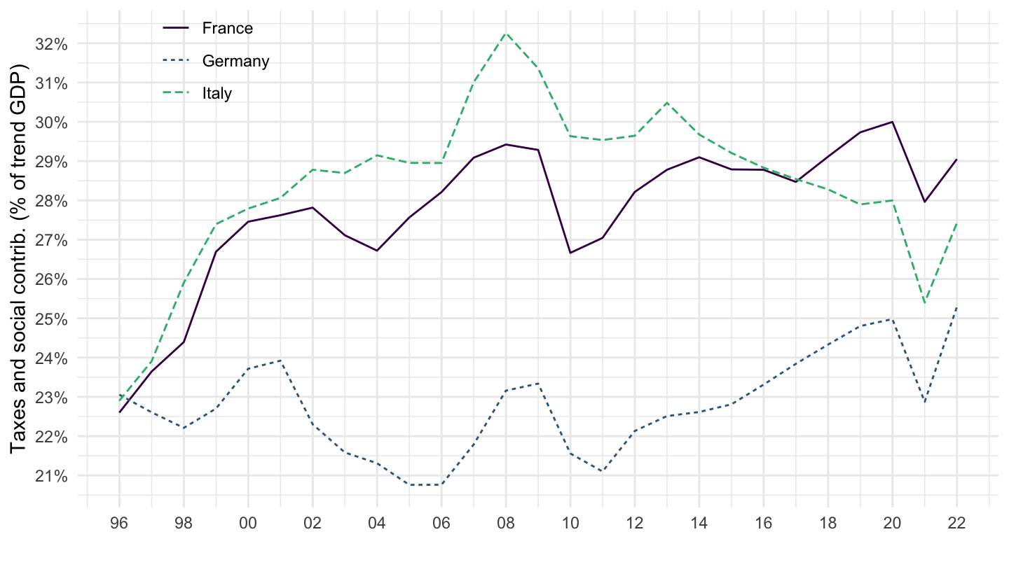

United Kingdom, Japan, United States

SNA_TABLE10 |>
  filter(TRANSACT %in% c("D2D5D91"),
         LOCATION %in% c("JPN", "GBR", "USA"),
         SECTOR == "TS13") |>
  left_join(SNA_TABLE1 |>
              filter(TRANSACT == "B1_GE",
                     MEASURE == "C") |>
              select(obsTime, LOCATION, B1_GE = obsValue), 
            by = c("LOCATION", "obsTime")) |>
  year_to_enddate() |>
  left_join(SNA_TABLE10_var$LOCATION |>
              setNames(c("LOCATION", "LOCATION_desc")), by = "LOCATION") |>
  select(LOCATION_desc, date, TRANSACT, obsValue, B1_GE) |>
  group_by(LOCATION_desc) |>
  mutate(B1_GE_trend = log(B1_GE) |> hpfilter(1000000) |> pluck("trend") |> exp(),
         obsValue = obsValue / B1_GE_trend) |>
  na.omit() |>
  ggplot() + geom_line(aes(x = date, y = obsValue, color = LOCATION_desc, linetype = LOCATION_desc)) +
  scale_color_manual(values = viridis(4)[1:3]) +
  theme_minimal() +
  scale_x_date(breaks = seq(1920, 2100, 2) |> paste0("-01-01") |> as.Date(),
               labels = date_format("%Y")) +
  theme(legend.position = c(0.15, 0.9),
        legend.title = element_blank()) +
  scale_y_continuous(breaks = 0.01*seq(-10, 100, 1),
                     labels = scales::percent_format(accuracy = 1)) +
  ylab("Taxes and social contrib. (% of trend GDP)") + xlab("")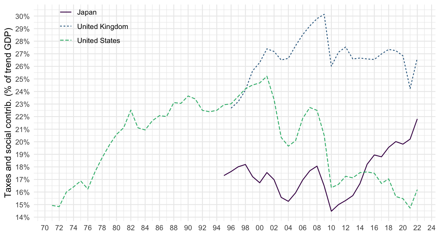

Switzerland, Germany, Netherlands

SNA_TABLE10 |>
  filter(TRANSACT %in% c("D2D5D91"),
         LOCATION %in% c("NLD", "CHE", "DEU"),
         SECTOR == "TS13") |>
  left_join(SNA_TABLE1 |>
              filter(TRANSACT == "B1_GE",
                     MEASURE == "C") |>
              select(obsTime, LOCATION, B1_GE = obsValue), 
            by = c("LOCATION", "obsTime")) |>
  year_to_enddate() |>
  left_join(SNA_TABLE10_var$LOCATION |>
              setNames(c("LOCATION", "LOCATION_desc")), by = "LOCATION") |>
  select(LOCATION_desc, date, TRANSACT, obsValue, B1_GE) |>
  group_by(LOCATION_desc) |>
  mutate(B1_GE_trend = log(B1_GE) |> hpfilter(1000000) |> pluck("trend") |> exp(),
         obsValue = obsValue / B1_GE_trend) |>
  na.omit() |>
  ggplot() + geom_line(aes(x = date, y = obsValue, color = LOCATION_desc, linetype = LOCATION_desc)) +
  scale_color_manual(values = viridis(4)[1:3]) +
  theme_minimal() +
  scale_x_date(breaks = seq(1920, 2100, 2) |> paste0("-01-01") |> as.Date(),
               labels = date_format("%Y")) +
  theme(legend.position = c(0.15, 0.9),
        legend.title = element_blank()) +
  scale_y_continuous(breaks = 0.01*seq(-10, 100, 1),
                     labels = scales::percent_format(accuracy = 1)) +
  ylab("Taxes and social contrib. (% of trend GDP)") + xlab("")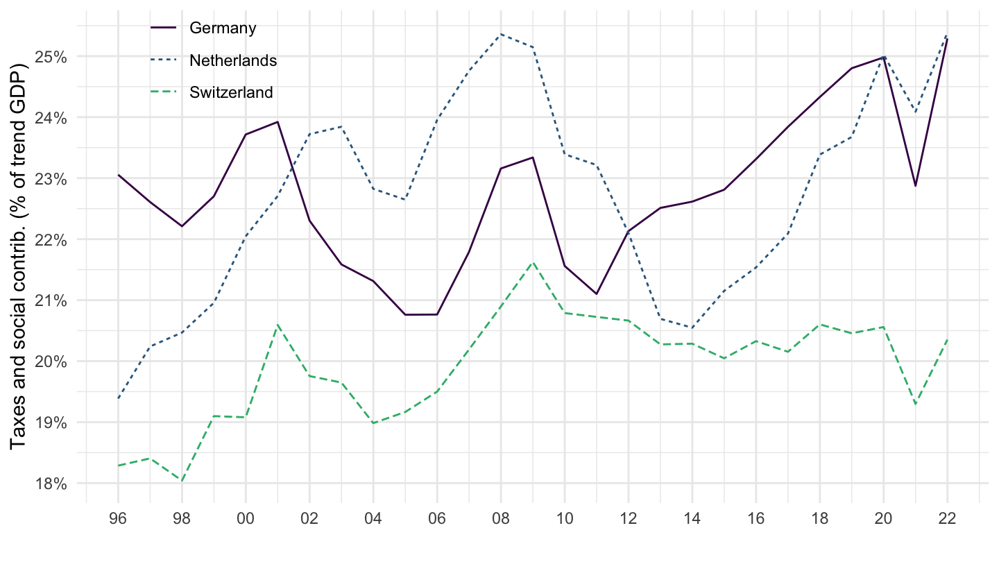

Ex: TAXB - Total receipts from taxes and social contrib

France, Germany, Italy

SNA_TABLE10 |>
  filter(TRANSACT %in% c("TAXB"),
         LOCATION %in% c("FRA", "DEU", "ITA"),
         SECTOR == "TS13") |>
  left_join(SNA_TABLE1 |>
              filter(TRANSACT == "B1_GE",
                     MEASURE == "C") |>
              select(obsTime, LOCATION, B1_GE = obsValue), 
            by = c("LOCATION", "obsTime")) |>
  year_to_enddate() |>
  left_join(SNA_TABLE10_var$LOCATION |>
              setNames(c("LOCATION", "LOCATION_desc")), by = "LOCATION") |>
  select(LOCATION_desc, date, TRANSACT, obsValue, B1_GE) |>
  group_by(LOCATION_desc) |>
  mutate(B1_GE_trend = log(B1_GE) |> hpfilter(1000000) |> pluck("trend") |> exp(),
         obsValue = obsValue / B1_GE_trend) |>
  na.omit() |>
  ggplot() + geom_line(aes(x = date, y = obsValue, color = LOCATION_desc, linetype = LOCATION_desc)) +
  scale_color_manual(values = viridis(4)[1:3]) +
  theme_minimal() +
  scale_x_date(breaks = seq(1920, 2100, 2) |> paste0("-01-01") |> as.Date(),
               labels = date_format("%Y")) +
  theme(legend.position = c(0.15, 0.9),
        legend.title = element_blank()) +
  scale_y_continuous(breaks = 0.01*seq(-10, 100, 1),
                     labels = scales::percent_format(accuracy = 1)) +
  ylab("Taxes and social contrib. (% of trend GDP)") + xlab("")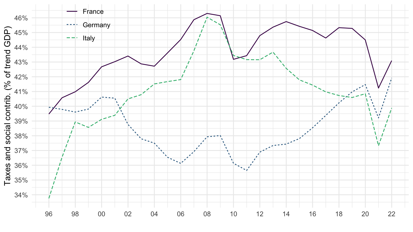

United Kingdom, Japan, United States

SNA_TABLE10 |>
  filter(TRANSACT %in% c("TAXB"),
         LOCATION %in% c("JPN", "GBR", "USA"),
         SECTOR == "TS13") |>
  left_join(SNA_TABLE1 |>
              filter(TRANSACT == "B1_GE",
                     MEASURE == "C") |>
              select(obsTime, LOCATION, B1_GE = obsValue), 
            by = c("LOCATION", "obsTime")) |>
  year_to_enddate() |>
  left_join(SNA_TABLE10_var$LOCATION |>
              setNames(c("LOCATION", "LOCATION_desc")), by = "LOCATION") |>
  select(LOCATION_desc, date, TRANSACT, obsValue, B1_GE) |>
  group_by(LOCATION_desc) |>
  mutate(B1_GE_trend = log(B1_GE) |> hpfilter(1000000) |> pluck("trend") |> exp(),
         obsValue = obsValue / B1_GE_trend) |>
  na.omit() |>
  ggplot() + geom_line(aes(x = date, y = obsValue, color = LOCATION_desc, linetype = LOCATION_desc)) +
  scale_color_manual(values = viridis(4)[1:3]) +
  theme_minimal() +
  scale_x_date(breaks = seq(1920, 2100, 2) |> paste0("-01-01") |> as.Date(),
               labels = date_format("%Y")) +
  theme(legend.position = c(0.15, 0.9),
        legend.title = element_blank()) +
  scale_y_continuous(breaks = 0.01*seq(-10, 100, 1),
                     labels = scales::percent_format(accuracy = 1)) +
  ylab("Taxes and social contrib. (% of trend GDP)") + xlab("")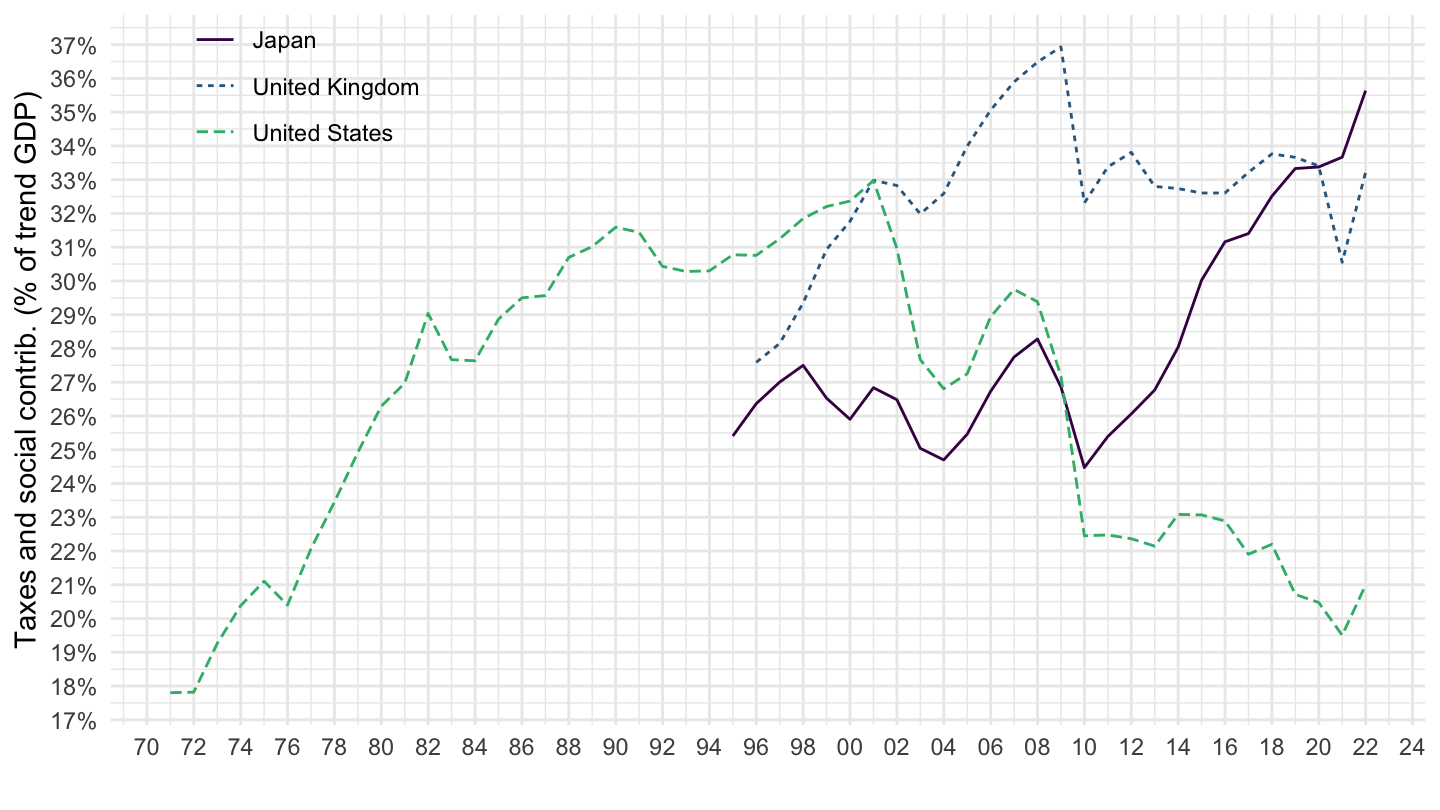

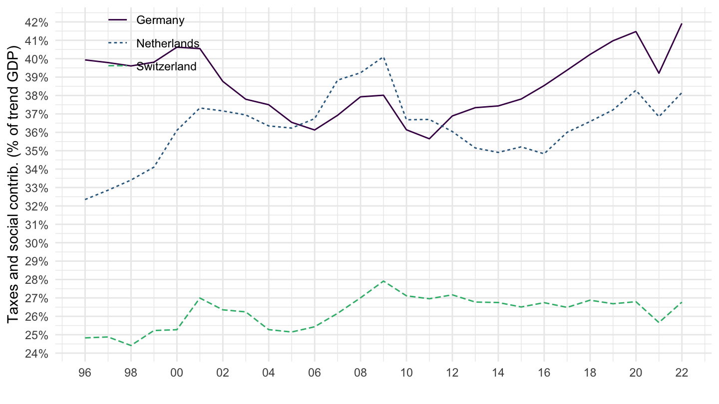
Switzerland, Germany, Netherlands

SNA_TABLE10 |>
  filter(TRANSACT %in% c("TAXB"),
         LOCATION %in% c("NLD", "CHE", "DEU"),
         SECTOR == "TS13") |>
  left_join(SNA_TABLE1 |>
              filter(TRANSACT == "B1_GE",
                     MEASURE == "C") |>
              select(obsTime, LOCATION, B1_GE = obsValue), 
            by = c("LOCATION", "obsTime")) |>
  year_to_enddate() |>
  left_join(SNA_TABLE10_var$LOCATION |>
              setNames(c("LOCATION", "LOCATION_desc")), by = "LOCATION") |>
  select(LOCATION_desc, date, TRANSACT, obsValue, B1_GE) |>
  group_by(LOCATION_desc) |>
  mutate(B1_GE_trend = log(B1_GE) |> hpfilter(1000000) |> pluck("trend") |> exp(),
         obsValue = obsValue / B1_GE_trend) |>
  na.omit() |>
  ggplot() + geom_line(aes(x = date, y = obsValue, color = LOCATION_desc, linetype = LOCATION_desc)) +
  scale_color_manual(values = viridis(4)[1:3]) +
  theme_minimal() +
  scale_x_date(breaks = seq(1920, 2100, 2) |> paste0("-01-01") |> as.Date(),
               labels = date_format("%Y")) +
  theme(legend.position = c(0.15, 0.9),
        legend.title = element_blank()) +
  scale_y_continuous(breaks = 0.01*seq(-10, 100, 1),
                     labels = scales::percent_format(accuracy = 1)) +
  ylab("Taxes and social contrib. (% of trend GDP)") + xlab("")