QNA - Japan - QNA_JPN
Data - OECD
Nobs - Quarterly - Javascript
Nobs - Annual - Javascript
LOCATION
SUBJECT
MEASURE
FREQUENCY
| FREQUENCY | Frequency | Nobs |
|---|---|---|
| Q | Quarterly | 40174 |
| A | Annual | 9683 |
obsTime
Japan’s boom-bust
Code
QNA %>%
  filter(LOCATION == "JPN",
         SUBJECT == "B1_GE",
         MEASURE == "VOBARSA",
         FREQUENCY == "Q") %>%
  quarter_to_date %>%
  filter(date >=  as.Date("1980-01-01"),
         date <= as.Date("2005-01-01")) %>%
  mutate(value = obsValue / 10^3) %>%
  select(date, value) %>%
  ggplot(aes(x = date, y = value)) + geom_line() + theme_minimal()  +
  scale_x_date(breaks = seq(1960, 2100, 5) %>% paste0("-01-01") %>% as.Date,
               labels = date_format("%Y")) +
  xlab("") + ylab("") +
  scale_y_log10(breaks = seq(0, 700000, 50000),
                labels = dollar_format(suffix = "Bn", prefix = "", accuracy = 1))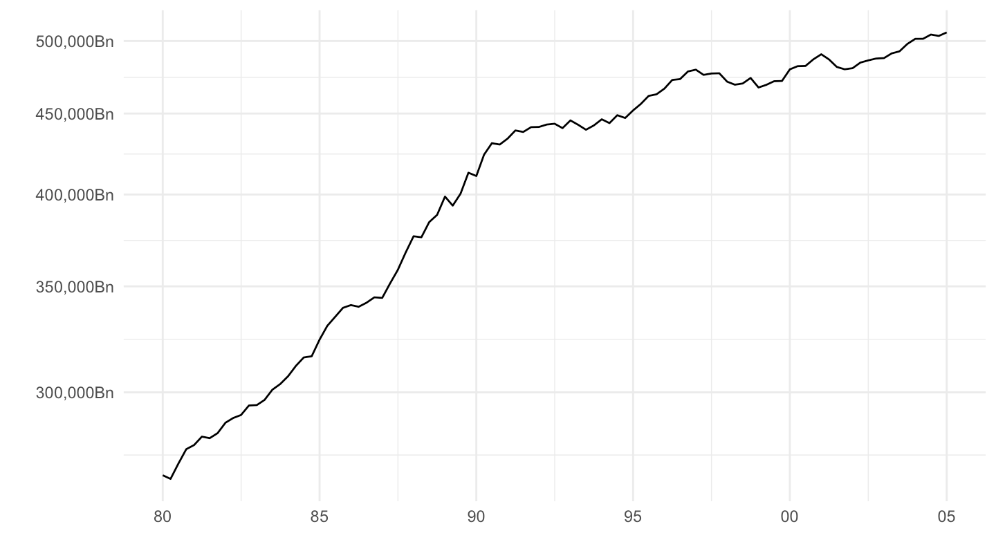
NX
1980-2005
Code
QNA %>%
  filter(LOCATION == "JPN",
         SUBJECT %in% c("P6", "P7"),
         MEASURE == "VOBARSA",
         FREQUENCY == "Q") %>%
  quarter_to_date %>%
  filter(date >=  as.Date("1980-01-01"),
         date <= as.Date("2005-01-01")) %>%
  mutate(value = obsValue / 10^3) %>%
  select(date, value, variable = SUBJECT) %>%
  spread(variable, value) %>%
  mutate(NX = P6 - P7) %>%
  ggplot(aes(x = date, y = NX)) + geom_line() + theme_minimal()  +
  scale_x_date(breaks = seq(1960, 2100, 5) %>% paste0("-01-01") %>% as.Date,
               labels = date_format("%Y")) +
  xlab("") + ylab("") +
  scale_y_continuous(breaks = seq(-20000, 20000, 2000),
                     labels = dollar_format(suffix = "Bn", prefix = "", accuracy = 1)) +
  geom_vline(xintercept = as.Date("1985-09-22"), linetype = "dashed", color = viridis(3)[2])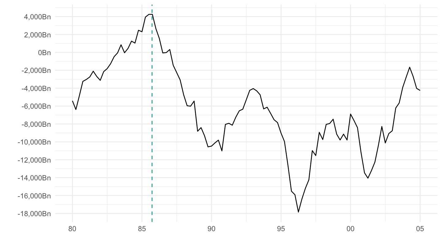
Japan
Code
QNA %>%
  filter(SUBJECT %in% c("P6", "P7", "B1_GE"),
         MEASURE == "VOBARSA",
         FREQUENCY == "Q",
         LOCATION %in% c("JPN")) %>%
  quarter_to_enddate %>%
  mutate(variable = paste0(SUBJECT, "_", MEASURE)) %>%
  left_join(QNA_var$LOCATION, by = "LOCATION") %>%
  select(Location, date, variable, obsValue) %>%
  spread(variable, obsValue) %>%
  mutate(NX_VOBARSA = (P6_VOBARSA - P7_VOBARSA) / B1_GE_VOBARSA) %>%
  ggplot() + geom_line() + theme_minimal() +
  aes(x = date, y = NX_VOBARSA) +
  scale_color_manual(values = viridis(4)[1:3]) +
  scale_x_date(breaks = seq(1920, 2100, 5) %>% paste0("-01-01") %>% as.Date,
               labels = date_format("%Y")) +
  theme(legend.position = c(0.15, 0.8),
        legend.title = element_blank()) +
  geom_hline(yintercept = 0, linetype = "dashed",  color = viridis(4)[3]) +
  scale_y_continuous(breaks = 0.01*seq(-20, 60, 2),
                     labels = scales::percent_format(accuracy = 1)) +
  ylab("% of GDP") + xlab("")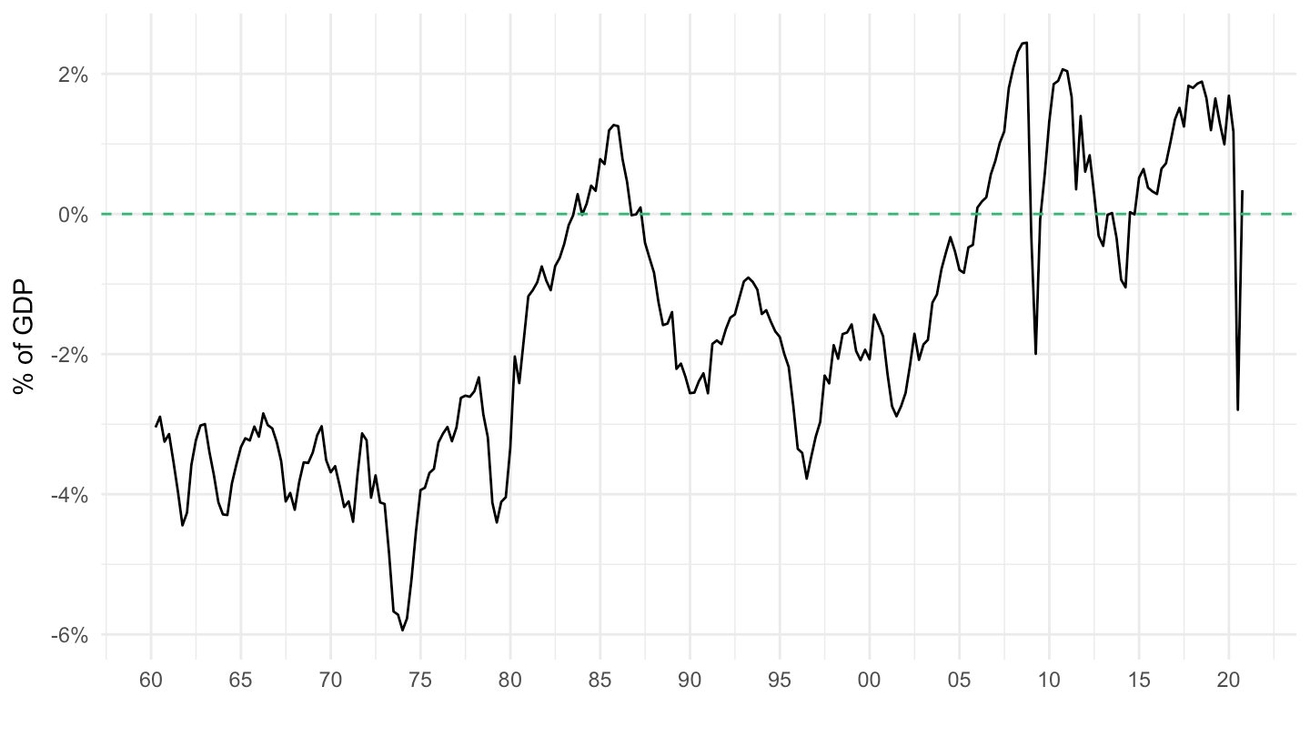
GDP: VOBARSA
1973-2007
(ref:JPN-B1-GE-73-07) Real GDP (1973-2007)
Code
QNA %>%
  filter(LOCATION == "JPN",
         SUBJECT == "B1_GE",
         MEASURE == "VOBARSA",
         FREQUENCY == "Q") %>%
  mutate(year = obsTime %>% substr(1, 4),
         qtr = obsTime %>% substr(7, 7) %>% as.numeric,
         month = (qtr - 1)*3 + 1,
         month = month %>% str_pad(., 2, pad = "0"),
         date = paste0(year, "-", month, "-01") %>% as.Date,
         value = obsValue / 10^3) %>%
  filter(date >= as.Date("1973-01-01"),
         date <= as.Date("2007-01-01")) %>%
  select(date, value) %>%
  ggplot(aes(x = date, y = value)) + geom_line() + theme_minimal()  +
  scale_x_date(breaks = seq(1960, 2100, 2) %>% paste0("-01-01") %>% as.Date,
               labels = date_format("%Y")) +
  xlab("") + ylab("") +
  scale_y_log10(breaks = seq(0, 700000, 50000),
                labels = dollar_format(suffix = "Bn", prefix = "", accuracy = 1))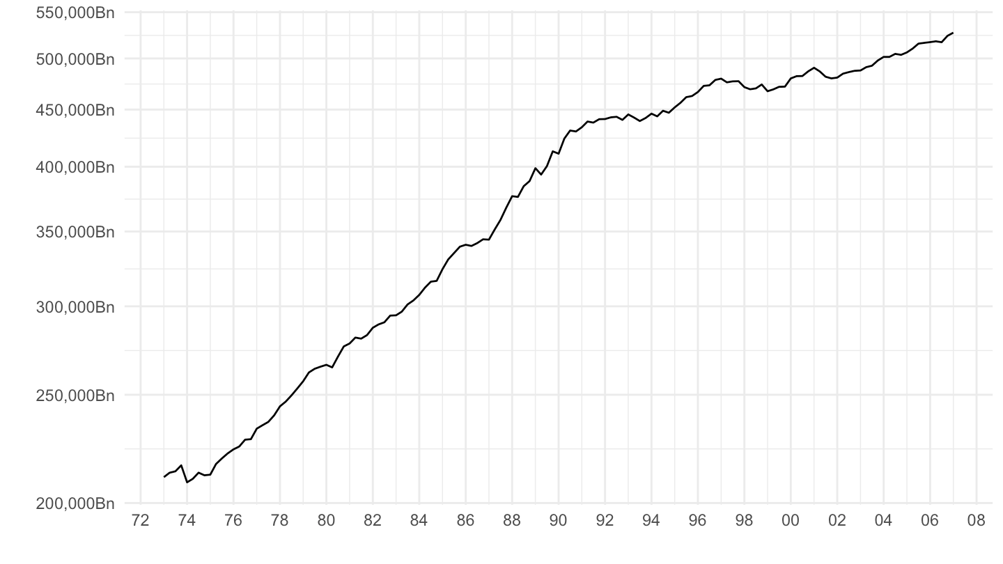
1984-2007
(ref:JPN-B1-GE-84-07) Real GDP (1984-2007)
Code
QNA %>%
  filter(LOCATION == "JPN",
         SUBJECT == "B1_GE",
         MEASURE == "VOBARSA",
         FREQUENCY == "Q") %>%
  mutate(year = obsTime %>% substr(1, 4),
         qtr = obsTime %>% substr(7, 7) %>% as.numeric,
         month = (qtr - 1)*3 + 1,
         month = month %>% str_pad(., 2, pad = "0"),
         date = paste0(year, "-", month, "-01") %>% as.Date,
         value = obsValue / 10^3) %>%
  filter(date >= as.Date("1984-01-01"),
         date <= as.Date("2007-01-01")) %>%
  select(date, value) %>%
  ggplot(aes(x = date, y = value)) + geom_line() + theme_minimal()  +
  scale_x_date(breaks = seq(1960, 2100, 2) %>% paste0("-01-01") %>% as.Date,
               labels = date_format("%Y")) +
  xlab("") + ylab("") +
  scale_y_log10(breaks = seq(0, 700000, 50000),
                labels = dollar_format(suffix = "Bn", prefix = "", accuracy = 1))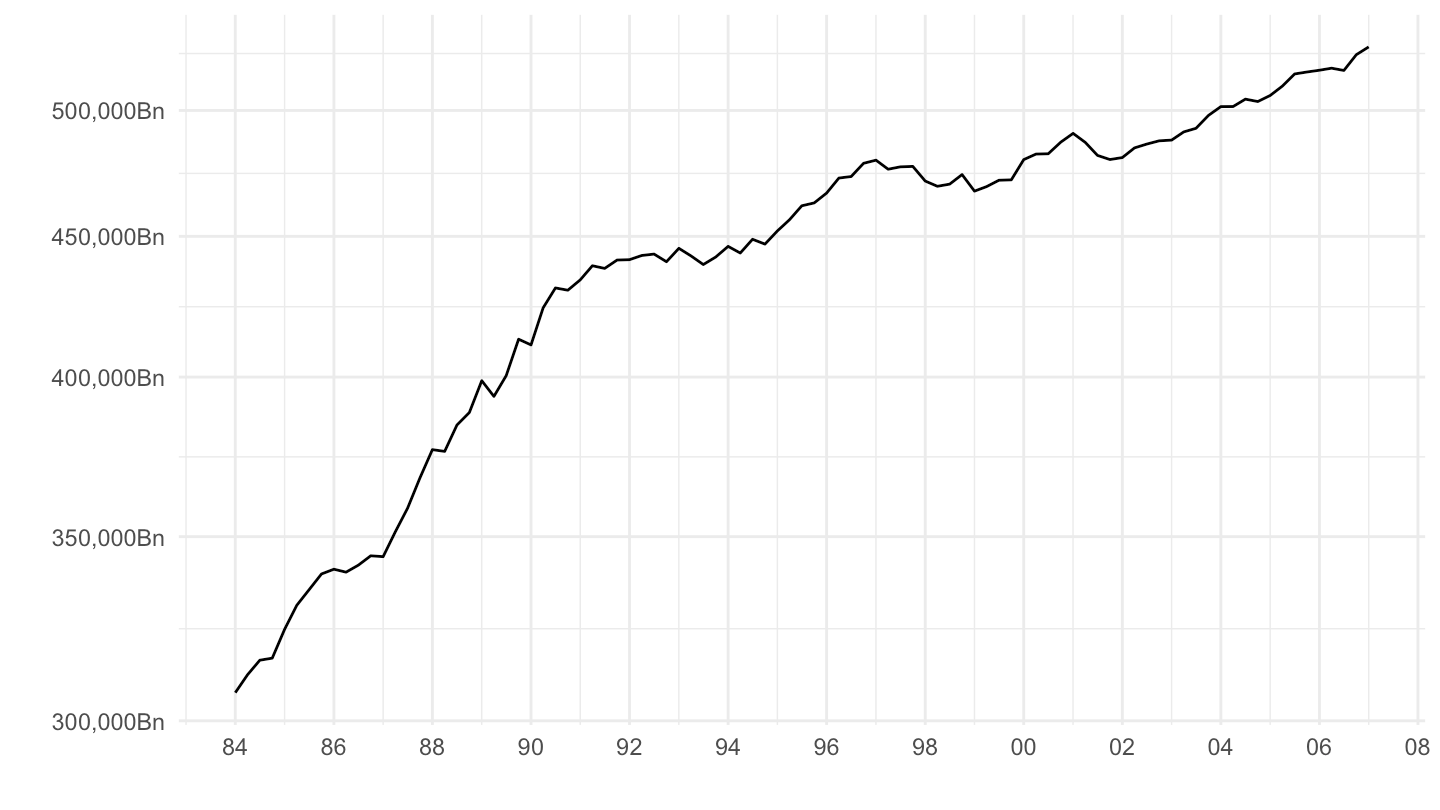
GDP: VPVOBARSA
1960-2007
(ref:JPN-B1-GE-60-07-VPVOBARSA) Real GDP (1960-2007)
Code
QNA %>%
  filter(LOCATION == "JPN",
         SUBJECT == "B1_GE",
         MEASURE == "VPVOBARSA",
         FREQUENCY == "Q") %>%
  quarter_to_date %>%
  mutate(value = obsValue / 10^3) %>%
  filter(date <= as.Date("2007-01-01")) %>%
  select(date, value) %>%
  ggplot(aes(x = date, y = value)) + geom_line() + theme_minimal()  +
  scale_x_date(breaks = seq(1960, 2100, 2) %>% paste0("-01-01") %>% as.Date,
               labels = date_format("%Y")) +
  xlab("") + ylab("") +
  scale_y_log10(breaks = seq(0, 7000, 500),
                labels = dollar_format(suffix = "Bn", prefix = "", accuracy = 1)) +
  geom_vline(xintercept = tax_JPN$date, linetype = "dashed", color = viridis(3)[2])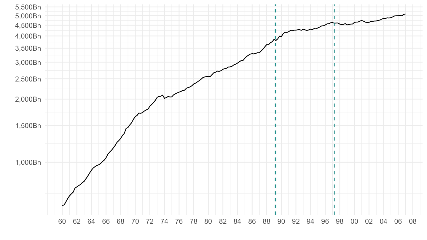
1973-2007
(ref:JPN-B1-GE-73-07-VPVOBARSA) Real GDP (1973-2007)
Code
QNA %>%
  filter(LOCATION == "JPN",
         SUBJECT == "B1_GE",
         MEASURE == "VPVOBARSA",
         FREQUENCY == "Q") %>%
  quarter_to_date %>%
  mutate(value = obsValue / 10^3) %>%
  filter(date >= as.Date("1973-01-01"),
         date <= as.Date("2007-01-01")) %>%
  select(date, value) %>%
  ggplot(aes(x = date, y = value)) + geom_line() + theme_minimal()  +
  scale_x_date(breaks = seq(1960, 2100, 2) %>% paste0("-01-01") %>% as.Date,
               labels = date_format("%Y")) +
  xlab("") + ylab("") +
  scale_y_log10(breaks = seq(0, 7000, 500),
                labels = dollar_format(suffix = "Bn", prefix = "", accuracy = 1)) +
  geom_vline(xintercept = tax_JPN$date, linetype = "dashed", color = viridis(3)[2])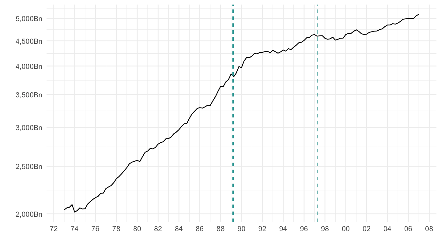
1984-2007
(ref:JPN-B1-GE-84-07-VPVOBARSA) Real GDP (1984-2007)
Code
QNA %>%
  filter(LOCATION == "JPN",
         SUBJECT == "B1_GE",
         MEASURE == "VPVOBARSA",
         FREQUENCY == "Q") %>%
  quarter_to_date %>%
  mutate(value = obsValue / 10^3) %>%
  filter(date >= as.Date("1984-01-01"),
         date <= as.Date("2007-01-01")) %>%
  select(date, value) %>%
  ggplot(aes(x = date, y = value)) + geom_line() + theme_minimal()  +
  scale_x_date(breaks = seq(1960, 2100, 2) %>% paste0("-01-01") %>% as.Date,
               labels = date_format("%Y")) +
  xlab("") + ylab("") +
  scale_y_log10(breaks = seq(0, 7000, 500),
                labels = dollar_format(suffix = "Bn", prefix = "", accuracy = 1)) +
  geom_vline(xintercept = tax_JPN$date, linetype = "dashed", color = viridis(3)[2])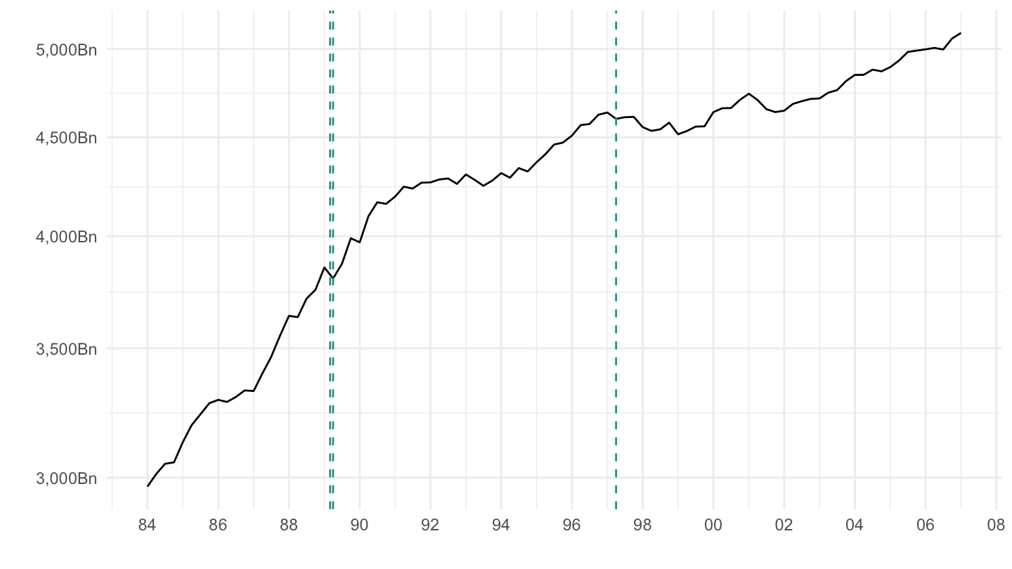
1984-2021
Code
QNA %>%
  filter(LOCATION == "JPN",
         SUBJECT == "B1_GE",
         MEASURE == "VPVOBARSA",
         FREQUENCY == "Q") %>%
  quarter_to_date %>%
  mutate(value = obsValue / 10^3) %>%
  filter(date >= as.Date("1984-01-01")) %>%
  select(date, value) %>%
  ggplot(aes(x = date, y = value)) + geom_line() + theme_minimal()  +
  scale_x_date(breaks = seq(1960, 2100, 2) %>% paste0("-01-01") %>% as.Date,
               labels = date_format("%Y")) +
  xlab("") + ylab("") +
  scale_y_log10(breaks = seq(0, 7000, 500),
                labels = dollar_format(suffix = "Bn", prefix = "", accuracy = 1)) +
  geom_vline(xintercept = tax_JPN$date, linetype = "dashed", color = viridis(3)[2])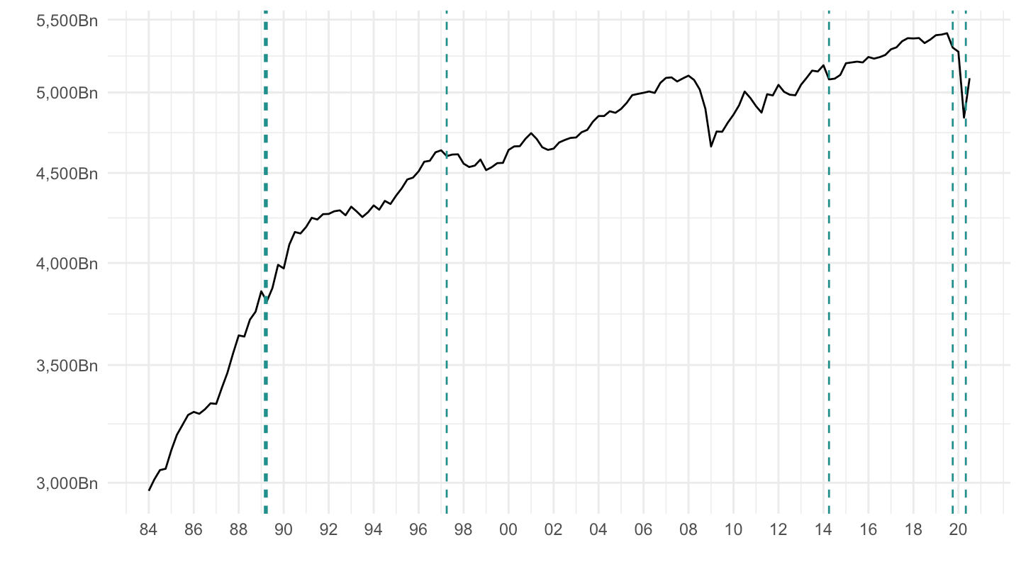
Plaza Accords
(ref:JPN-X-M-GDP) Exports and Imports, Japan (percentage of GDP)
Code
QNA %>%
  filter(SUBJECT %in% c("P6", "P7", "B1_GE"),
         MEASURE == "VOBARSA",
         FREQUENCY == "Q",
         LOCATION == "JPN") %>%
  quarter_to_date %>%
  mutate(variable = paste0(SUBJECT, "_", MEASURE)) %>%
  select(date, variable, obsValue) %>%
  spread(variable, obsValue) %>%
  mutate(`Exports (% of GDP)` = P6_VOBARSA / B1_GE_VOBARSA,
         `Imports (% of GDP)` = P7_VOBARSA / B1_GE_VOBARSA) %>%
  na.omit %>%
  select(-contains("VOBARSA")) %>%
  gather(variable, value, - date) %>%
  ggplot() + geom_line(aes(x = date, y = value, color = variable, linetype = variable)) +
  scale_color_manual(values = viridis(4)[1:3]) +
  theme_minimal() +
  scale_x_date(breaks = seq(1920, 2100, 5) %>% paste0("-01-01") %>% as.Date,
               labels = date_format("%Y")) +
  theme(legend.position = c(0.2, 0.9),
        legend.title = element_blank()) +
  geom_vline(xintercept = as.Date("1985-09-22"), linetype = "dashed", color = viridis(4)[3]) +
  scale_y_continuous(breaks = 0.01*seq(0, 60, 5),
                     labels = scales::percent_format(accuracy = 1)) +
  ylab("% of GDP (Japan)") + xlab("")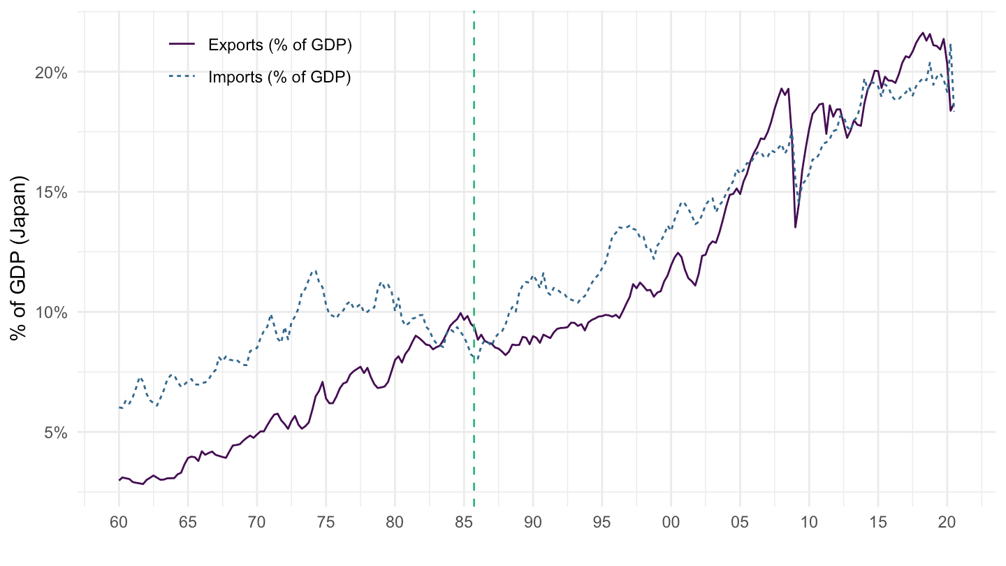
Other details
(ref:JPN-X-M-GDP-dates) Exports and Imports, Japan (% of GDP)
Code
QNA %>%
  filter(SUBJECT %in% c("P6", "P7", "B1_GE"),
         MEASURE == "VOBARSA",
         FREQUENCY == "Q",
         LOCATION == "JPN") %>%
  quarter_to_date %>%
  mutate(variable = paste0(SUBJECT, "_", MEASURE)) %>%
  select(date, variable, obsValue) %>%
  spread(variable, obsValue) %>%
  mutate(`Exports (% of GDP)` = P6_VOBARSA / B1_GE_VOBARSA,
         `Imports (% of GDP)` = P7_VOBARSA / B1_GE_VOBARSA) %>%
  na.omit %>%
  select(-contains("VOBARSA")) %>%
  gather(variable, value, - date) %>%
  ggplot() + geom_line(aes(x = date, y = value, color = variable, linetype = variable)) +
  scale_color_manual(values = viridis(4)[1:3]) +
  theme_minimal() +
  scale_x_date(breaks = seq(1920, 2100, 5) %>% paste0("-01-01") %>% as.Date,
               labels = date_format("%Y")) +
  theme(legend.position = c(0.2, 0.9),
        legend.title = element_blank()) +
  geom_vline(xintercept = as.Date(c("1985-09-22",
                                    "1989-04-01",
                                    "1997-04-01",
                                    "2014-04-01",
                                    "2019-10-01")),
             linetype = "dashed", color = viridis(4)[3]) +
  geom_rect(data = data_frame(start = as.Date("1979-06-01"),
                                end = as.Date("1985-09-22")),
              aes(xmin = start, xmax = end, ymin = -Inf, ymax = +Inf),
              fill = viridis(4)[4], alpha = 0.2) +
  scale_y_continuous(breaks = 0.01*seq(0, 60, 2),
                     labels = scales::percent_format(accuracy = 1)) +
  ylab("% of GDP (Japan)") + xlab("")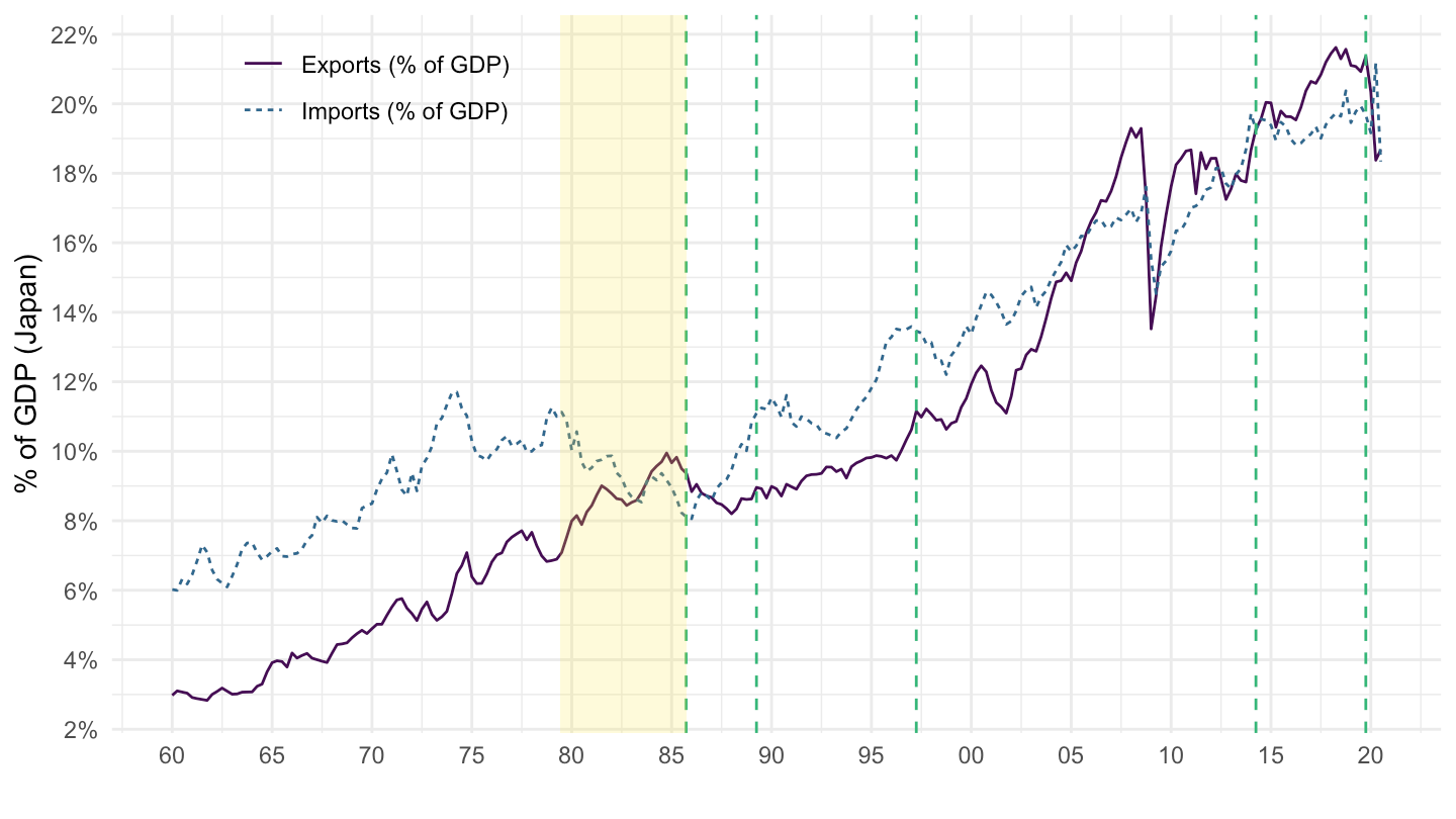
CA = S-I
All
Code
QNA %>%
  filter(SUBJECT %in% c("P6", "P7", "P51", "B1_GE"),
         MEASURE == "VOBARSA",
         FREQUENCY == "Q",
         LOCATION == "JPN") %>%
  quarter_to_date %>%
  mutate(variable = paste0(SUBJECT, "_", MEASURE)) %>%
  select(date, variable, obsValue) %>%
  spread(variable, obsValue) %>%
  mutate(`Saving (% of GDP)` = (P6_VOBARSA - P7_VOBARSA + P51_VOBARSA) / B1_GE_VOBARSA,
         `Investment (% of GDP)` = P51_VOBARSA / B1_GE_VOBARSA) %>%
  na.omit %>%
  select(-contains("VOBARSA")) %>%
  gather(variable, value, - date) %>%
  ggplot() + geom_line(aes(x = date, y = value, color = variable, linetype = variable)) +
  scale_color_manual(values = viridis(4)[1:3]) +
  theme_minimal() +
  scale_x_date(breaks = seq(1920, 2100, 5) %>% paste0("-01-01") %>% as.Date,
               labels = date_format("%Y")) +
  theme(legend.position = c(0.45, 0.9),
        legend.title = element_blank()) +
  scale_y_continuous(breaks = 0.01*seq(-7, 60, 1),
                     labels = scales::percent_format(accuracy = 1)) +
  ylab("% of GDP") + xlab("") +
  geom_vline(xintercept = tax_JPN$date, linetype = "dashed", color = viridis(3)[2])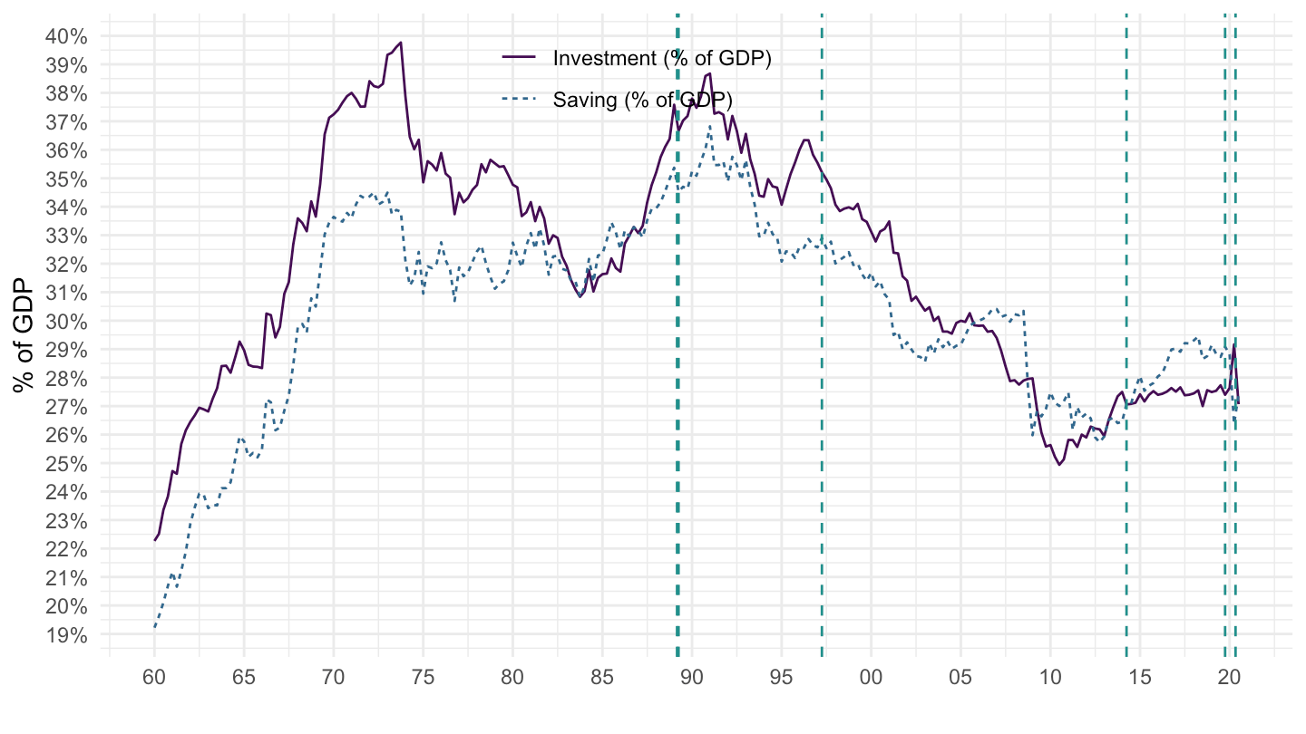
All
Code
QNA %>%
  filter(SUBJECT %in% c("P6", "P7", "P51", "B1_GE"),
         MEASURE == "VOBARSA",
         FREQUENCY == "Q",
         LOCATION == "JPN") %>%
  quarter_to_date %>%
  mutate(variable = paste0(SUBJECT, "_", MEASURE)) %>%
  select(date, variable, obsValue) %>%
  spread(variable, obsValue) %>%
  mutate(`Saving (% of GDP)` = (P6_VOBARSA - P7_VOBARSA + P51_VOBARSA) / B1_GE_VOBARSA,
         `Investment (% of GDP)` = P51_VOBARSA / B1_GE_VOBARSA) %>%
  na.omit %>%
  select(-contains("VOBARSA")) %>%
  gather(variable, value, - date) %>%
  ggplot() + geom_line(aes(x = date, y = value, color = variable, linetype = variable)) +
  scale_color_manual(values = viridis(4)[1:3]) +
  theme_minimal() +
  scale_x_date(breaks = seq(1920, 2100, 5) %>% paste0("-01-01") %>% as.Date,
               labels = date_format("%Y")) +
  theme(legend.position = c(0.45, 0.9),
        legend.title = element_blank()) +
  scale_y_continuous(breaks = 0.01*seq(-7, 60, 1),
                     labels = scales::percent_format(accuracy = 1)) +
  ylab("% of GDP") + xlab("")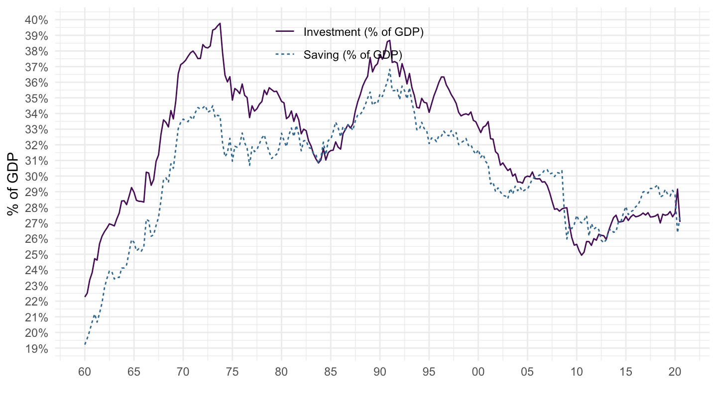
Exports and Imports (% of GDP)
Code
QNA %>%
  filter(LOCATION == "JPN",
         SUBJECT %in% c("P6", "P7"),
         MEASURE == "VOBARSA",
         FREQUENCY == "Q") %>%
  quarter_to_date %>%
  mutate(value = obsValue / 10^3) %>%
  filter(date >= as.Date("1987-01-01"),
         date <= as.Date("2000-01-01")) %>%
  select(date, value, variable = SUBJECT) %>%
  mutate(Variable = case_when(variable == "P6" ~ "Exports",
                                   variable == "P7" ~ "Imports")) %>%
  ggplot() + geom_line(aes(x = date, y = value, color = Variable, linetype = Variable)) +
  scale_color_manual(values = viridis(4)[1:3]) +
  theme_minimal() +
  scale_x_date(breaks = as.Date(paste0(seq(1960, 2020, 1), "-01-01")),
               labels = date_format("%Y")) +
  theme(legend.position = c(0.2, 0.85),
        legend.title = element_blank()) +
  xlab("") + ylab("") +
  scale_y_log10(breaks = seq(0, 80000, 5000),
                labels = dollar_format(a = 1, p = "¥ ", su = " Bn"))
X, M (1970-2020)
Code
QNA %>%
  filter(LOCATION == "JPN",
         SUBJECT %in% c("P6", "P7"),
         MEASURE == "VOBARSA",
         FREQUENCY == "Q") %>%
  quarter_to_date %>%
  mutate(value = obsValue / 10^3) %>%
  filter(date >= as.Date("1970-01-01"),
         date <= as.Date("2020-01-01")) %>%
  select(date, value, variable = SUBJECT) %>%
  mutate(Variable = case_when(variable == "P6" ~ "Exports",
                                   variable == "P7" ~ "Imports")) %>%
  ggplot() + geom_line(aes(x = date, y = value, color = Variable, linetype = Variable)) +
  scale_color_manual(values = viridis(4)[1:3]) +
  theme_minimal() +
  scale_x_date(breaks = as.Date(paste0(seq(1960, 2020, 5), "-01-01")),
               labels = date_format("%Y")) +
  theme(legend.position = c(0.2, 0.85),
        legend.title = element_blank()) +
  xlab("") + ylab("") +
  scale_y_log10(breaks = seq(0, 120000, 10000),
                labels = dollar_format(a = 1, p = "¥ ", su = " Bn"))
X, M (2010-2020)
Code
QNA %>%
  filter(LOCATION == "JPN",
         SUBJECT %in% c("P6", "P7"),
         MEASURE == "VOBARSA",
         FREQUENCY == "Q") %>%
  quarter_to_date %>%
  mutate(value = obsValue / 10^3) %>%
  filter(date >= as.Date("2010-01-01"),
         date <= as.Date("2020-01-01")) %>%
  select(date, value, variable = SUBJECT) %>%
  mutate(Variable = case_when(variable == "P6" ~ "Exports",
                                   variable == "P7" ~ "Imports")) %>%
  ggplot() + geom_line(aes(x = date, y = value, color = Variable, linetype = Variable)) +
  scale_color_manual(values = viridis(4)[1:3]) +
  theme_minimal() +
  scale_x_date(breaks = as.Date(paste0(seq(1960, 2020, 1), "-01-01")),
               labels = date_format("%Y")) +
  theme(legend.position = c(0.2, 0.85),
        legend.title = element_blank()) +
  xlab("") + ylab("") +
  scale_y_log10(breaks = seq(0, 120000, 10000),
                labels = dollar_format(a = 1, p = "¥ ", su = " Bn"))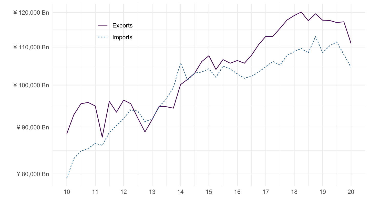
X, M (1976-1990)
Code
QNA %>%
  filter(LOCATION == "JPN",
         SUBJECT %in% c("P6", "P7"),
         MEASURE == "VOBARSA",
         FREQUENCY == "Q") %>%
  quarter_to_date %>%
  mutate(value = obsValue / 10^3) %>%
  filter(date >= as.Date("1976-01-01"),
         date <= as.Date("1990-01-01")) %>%
  select(date, value, variable = SUBJECT) %>%
  mutate(Variable = case_when(variable == "P6" ~ "Exports",
                                   variable == "P7" ~ "Imports")) %>%
  ggplot() + geom_line(aes(x = date, y = value, color = Variable, linetype = Variable)) +
  scale_color_manual(values = viridis(4)[1:3]) +
  theme_minimal() +
  scale_x_date(breaks = as.Date(paste0(seq(1960, 2020, 1), "-01-01")),
               labels = date_format("%Y")) +
  theme(legend.position = c(0.2, 0.85),
        legend.title = element_blank()) +
  xlab("") + ylab("") +
  scale_y_log10(breaks = seq(0, 80000, 5000),
                labels = dollar_format(a = 1, p = "¥ ", su = " Bn"))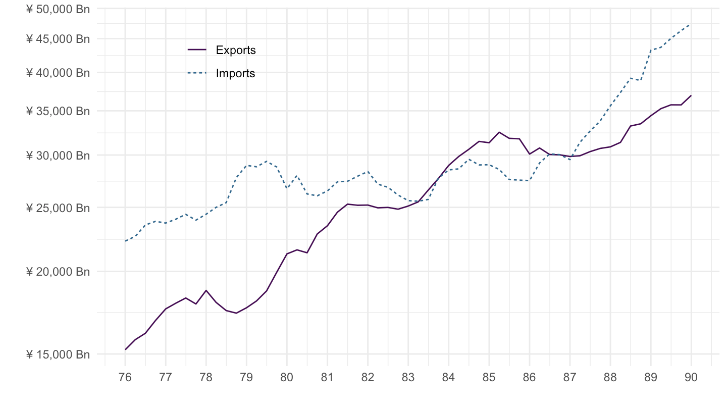
Consumption
2012-
Code
QNA %>%
  filter(LOCATION == "JPN",
         SUBJECT == "P31S14_S15",
         MEASURE == "VOBARSA",
         FREQUENCY == "Q") %>%
  quarter_to_date %>%
  mutate(value = obsValue / 10^3) %>%
  filter(date >= as.Date("2012-01-01")) %>%
  select(date, value, variable = SUBJECT) %>%
  ggplot() + geom_line(aes(x = date, y = value)) + theme_minimal()  +
  scale_x_date(breaks = as.Date(paste0(seq(1960, 2020, 1), "-01-01")),
               labels = date_format("%Y")) +
  xlab("") + ylab("Consumption in Japan") +
  scale_y_continuous(breaks = seq(0, 600000, 1000),
                labels = dollar_format(a = 1, p = "¥ ", su = " Bn"))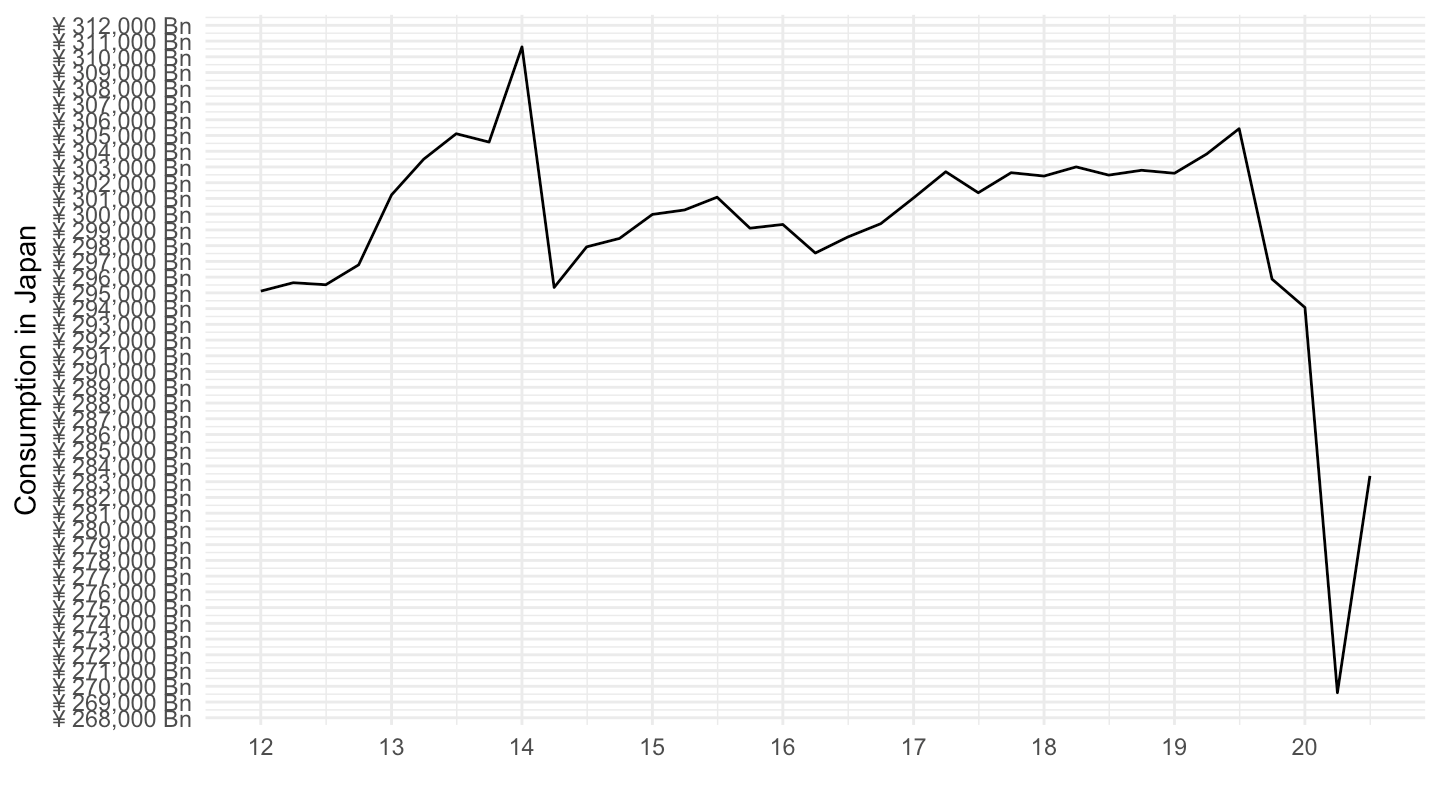
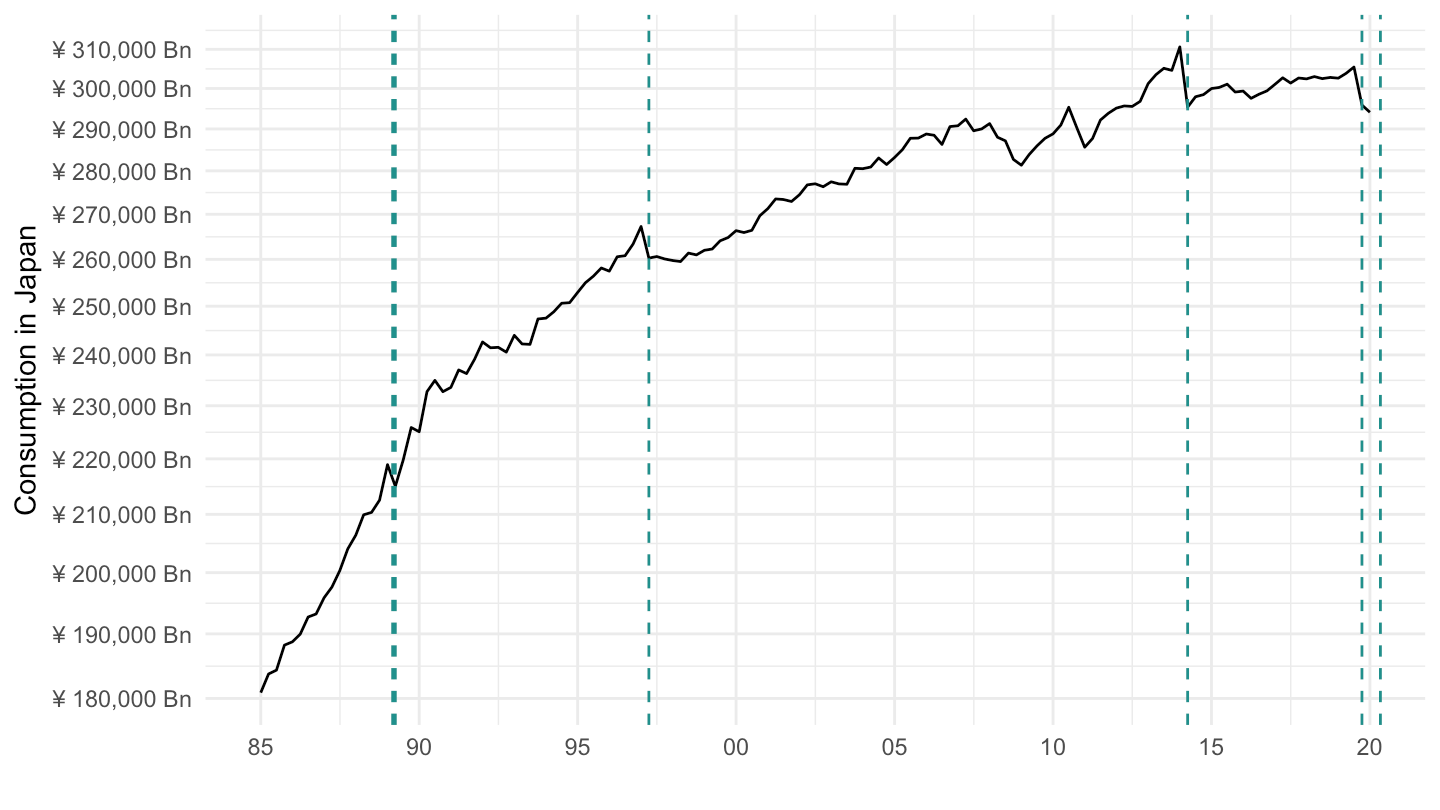
1985-
Code
QNA %>%
  filter(LOCATION == "JPN",
         SUBJECT == "P31S14_S15",
         MEASURE == "VOBARSA",
         FREQUENCY == "Q") %>%
  quarter_to_date %>%
  mutate(value = obsValue / 10^3) %>%
  filter(date >= as.Date("1985-01-01"),
         date <= as.Date("2020-01-01")) %>%
  select(date, value, variable = SUBJECT) %>%
  ggplot() + geom_line(aes(x = date, y = value)) + theme_minimal()  +
  scale_x_date(breaks = as.Date(paste0(seq(1960, 2020, 5), "-01-01")),
               labels = date_format("%Y")) +
  xlab("") + ylab("Consumption in Japan") +
  scale_y_log10(breaks = seq(0, 600000, 10000),
                labels = dollar_format(a = 1, p = "¥ ", su = " Bn")) +
  geom_vline(xintercept = tax_JPN$date, linetype = "dashed", color = viridis(3)[2])