Quarterly National Accounts (Archive before 2019 benchmark revisions) - QNA_ARCHIVE
Data - OECD
Nobs - Quarterly - Javascript
Nobs - Annual - Javascript
Data Structure
| id | description |
|---|---|
| LOCATION | Country |
| SUBJECT | Subject |
| MEASURE | Measure |
| FREQUENCY | Frequency |
| TIME | Period |
| OBS_VALUE | Observation Value |
| TIME_FORMAT | Time Format |
| OBS_STATUS | Observation Status |
| UNIT | Unit |
| POWERCODE | Unit multiplier |
| REFERENCEPERIOD | Reference period |
SUBJECT
MEASURE
FREQUENCY
| id | label |
|---|---|
| A | Annual |
| Q | Quarterly |
TIME_FORMAT
| id | label |
|---|---|
| P1Y | Annual |
| P1M | Monthly |
| P3M | Quarterly |
| P6M | Half-yearly |
| P1D | Daily |
UNIT
POWERCODE
REFERENCEPERIOD
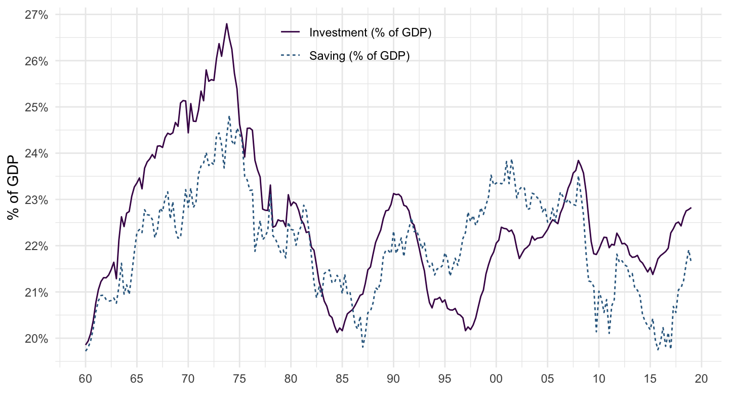
Example 1A: Germany’s CA = S-I
Code
QNA_ARCHIVE %>%
  filter(SUBJECT %in% c("P6", "P7", "P51", "B1_GE"),
         MEASURE == "VOBARSA",
         FREQUENCY == "Q",
         LOCATION == "DEU") %>%
  quarter_to_date %>%
  mutate(variable = paste0(SUBJECT, "_", MEASURE)) %>%
  select(date, variable, obsValue) %>%
  spread(variable, obsValue) %>%
  mutate(`Saving (% of GDP)` = (P6_VOBARSA - P7_VOBARSA + P51_VOBARSA) / B1_GE_VOBARSA,
         `Investment (% of GDP)` = P51_VOBARSA / B1_GE_VOBARSA) %>%
  na.omit %>%
  select(-contains("VOBARSA")) %>%
  gather(variable, value, - date) %>%
  ggplot() + geom_line(aes(x = date, y = value, color = variable, linetype = variable)) +
  scale_color_manual(values = viridis(4)[1:3]) +
  theme_minimal() +
  scale_x_date(breaks = seq(1920, 2025, 5) %>% paste0("-01-01") %>% as.Date,
               labels = date_format("%y")) +
  theme(legend.position = c(0.45, 0.9),
        legend.title = element_blank()) +
  scale_y_continuous(breaks = 0.01*seq(-7, 60, 1),
                     labels = scales::percent_format(accuracy = 1)) +
  ylab("% of GDP") + xlab("")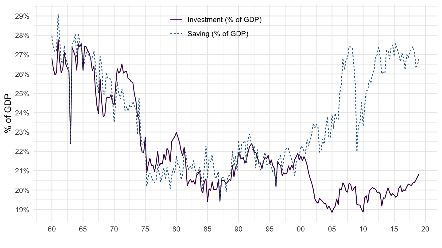
Example 1B: Exports and Imports in Germany (Value)
Code
QNA_ARCHIVE %>%
  filter(LOCATION == "DEU",
         SUBJECT %in% c("P6", "P7"),
         MEASURE == "VOBARSA",
         FREQUENCY == "Q") %>%
  quarter_to_date %>%
  mutate(value = obsValue / 10^3) %>%
  filter(date >= as.Date("1960-01-01"),
         date <= as.Date("2020-01-01")) %>%
  select(date, value, variable = SUBJECT) %>%
  mutate(variable_desc = case_when(variable == "P6" ~ "Exports",
                                   variable == "P7" ~ "Imports")) %>%
  ggplot() + geom_line(aes(x = date, y = value, color = variable_desc, linetype = variable_desc)) +
  scale_color_manual(values = viridis(4)[1:3]) +
  theme_minimal() +
  scale_x_date(breaks = as.Date(paste0(seq(1960, 2020, 5), "-01-01")),
               labels = date_format("%y")) +
  theme(legend.position = c(0.2, 0.85),
        legend.title = element_blank()) +
  xlab("") + ylab("") +
  scale_y_log10(breaks = seq(0, 2000, 100),
                labels = dollar_format(suffix = " Bn€", prefix = "", accuracy = 1))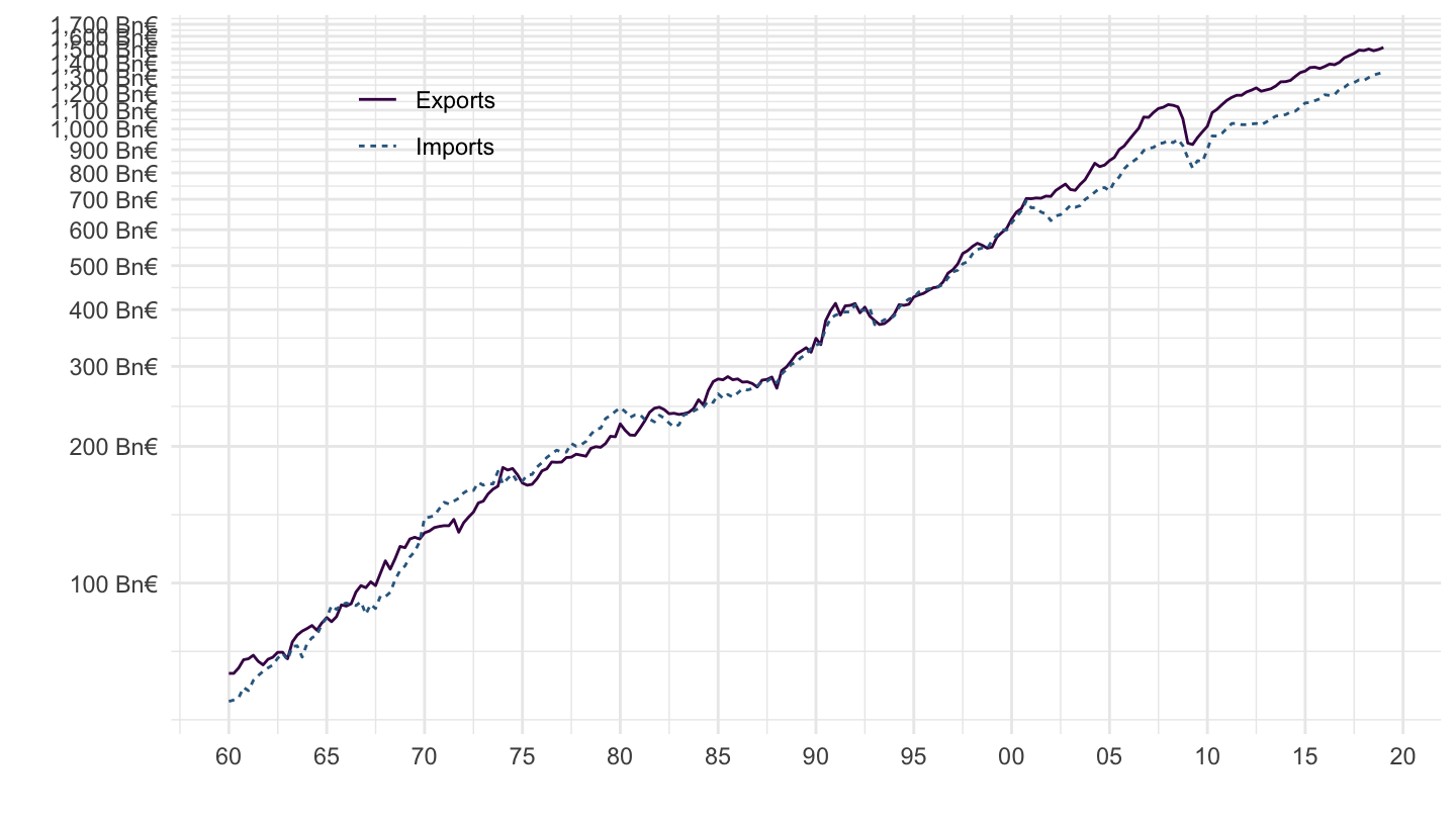
Example 1C: Exports and Imports in Germany (% of GDP)
Code
QNA_ARCHIVE %>%
  filter(SUBJECT %in% c("P6", "P7", "B1_GE"),
         MEASURE == "VOBARSA",
         FREQUENCY == "Q",
         LOCATION == "DEU") %>%
  quarter_to_date %>%
  mutate(variable = paste0(SUBJECT, "_", MEASURE)) %>%
  select(date, variable, obsValue) %>%
  spread(variable, obsValue) %>%
  mutate(`Exports (% of GDP)` = P6_VOBARSA / B1_GE_VOBARSA,
         `Imports (% of GDP)` = P7_VOBARSA / B1_GE_VOBARSA) %>%
  na.omit %>%
  select(-contains("VOBARSA")) %>%
  gather(variable, value, - date) %>%
  ggplot() + geom_line(aes(x = date, y = value, color = variable, linetype = variable)) +
  scale_color_manual(values = viridis(4)[1:3]) +
  theme_minimal() +
  scale_x_date(breaks = seq(1920, 2025, 5) %>% paste0("-01-01") %>% as.Date,
               labels = date_format("%y")) +
  theme(legend.position = c(0.45, 0.9),
        legend.title = element_blank()) +
  scale_y_continuous(breaks = 0.01*seq(0, 60, 5),
                     labels = scales::percent_format(accuracy = 1)) +
  ylab("% of GDP") + xlab("")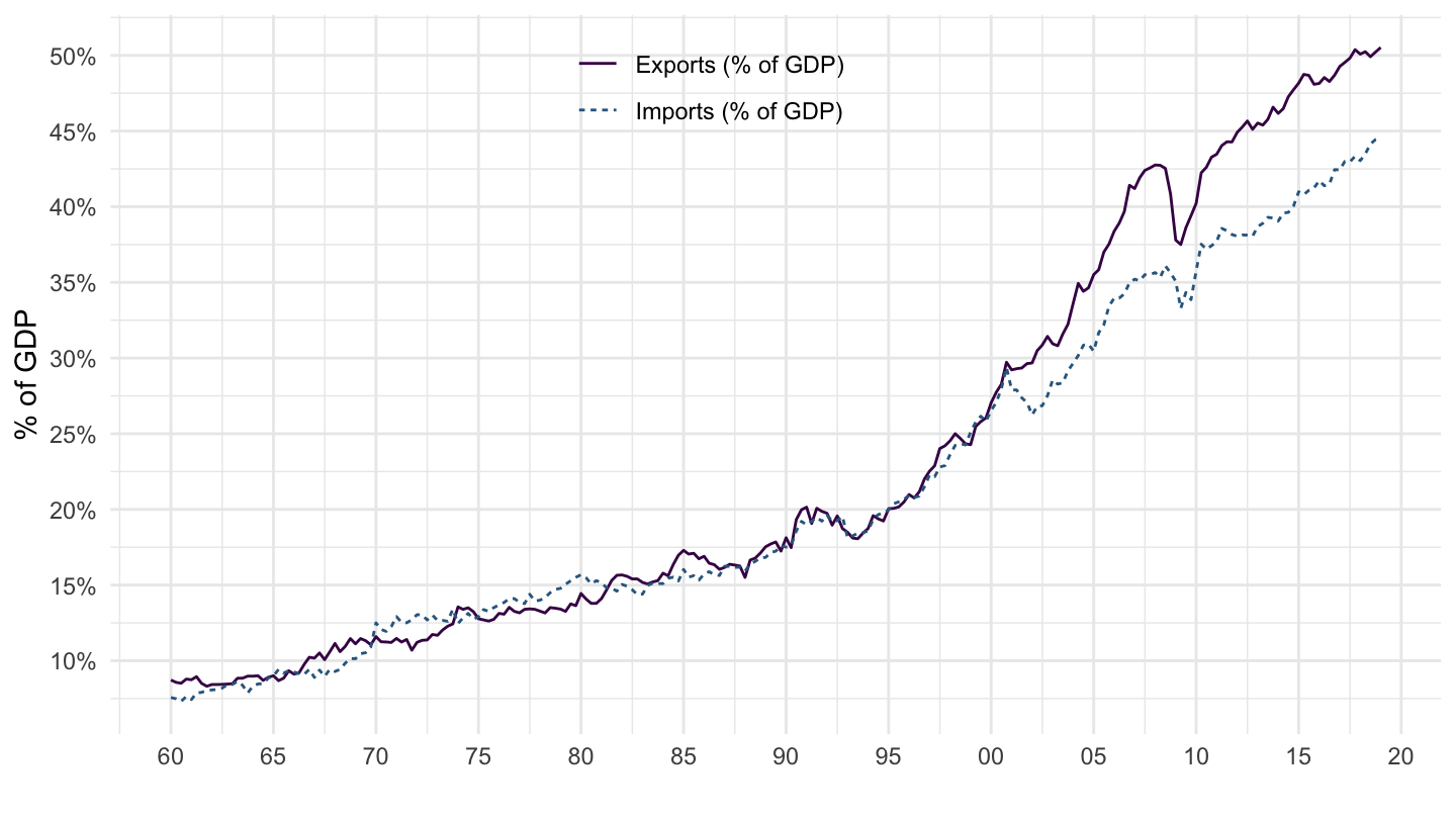
Example 2: GDP Plot
Code
QNA_ARCHIVE %>%
  filter(SUBJECT == "B1_GE",
         MEASURE == "VOBARSA",
         FREQUENCY == "Q",
         LOCATION == "FRA") %>%
  quarter_to_date %>%
  select(date, obsValue) %>%
  mutate(obsValue = obsValue / 1000000,
         yearqtr = year(date) + (month(date)-1)/12) %>%
  mutate(`HP 1000` = log(obsValue) %>% hpfilter(1000) %>% pluck("trend") %>% exp,
         `HP 1000000` = log(obsValue) %>% hpfilter(1000000) %>% pluck("trend") %>% exp,
         `Log` = lm(log(obsValue) ~ yearqtr) %>% fitted %>% exp) %>%
  group_by(date) %>%
  select(-yearqtr) %>%
  gather(variable, value, -date) %>%
  ggplot(.) + geom_line(aes(x = date, y = value, color = variable)) +
  theme_minimal() + scale_color_manual(values = viridis(5)[1:4]) +
  theme(legend.title = element_blank(),
        legend.position = c(0.8, 0.2)) +
  scale_x_date(breaks = seq(1950, 2020, 5) %>% paste0("-01-01") %>% as.Date,
               labels = date_format("%y")) +
  scale_y_log10(breaks = 20*2^seq(-7, 1, 0.5),
                labels = dollar_format(accuracy = 0.1, suffix = "Tn€", prefix = "")) +
  xlab("") + ylab("Real GDP (France)")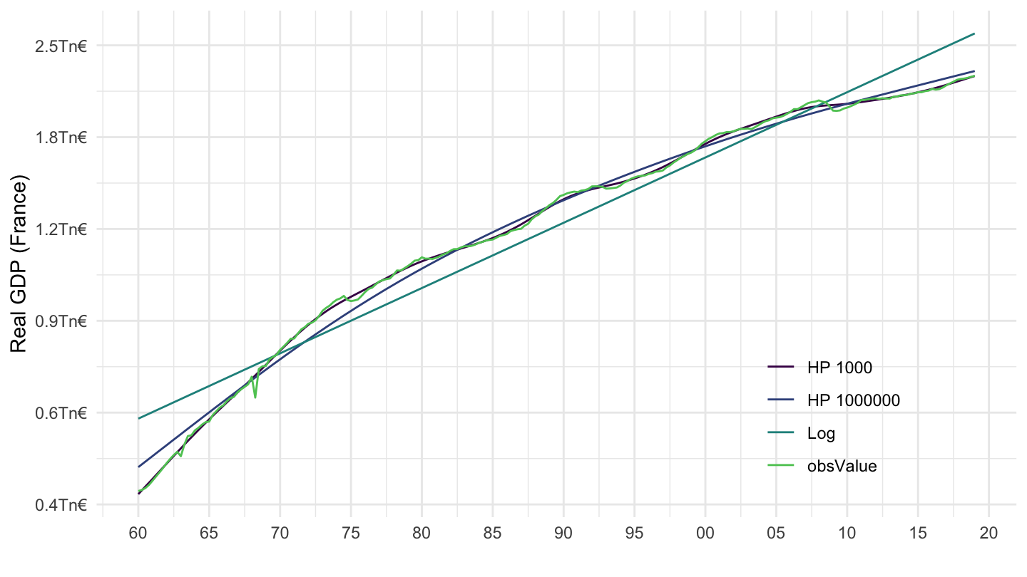
Example 3: Net saving in France and Germany
Code
QNA_ARCHIVE %>%
  filter(SUBJECT == "B8NS1",
         MEASURE == "CQR",
         FREQUENCY == "Q",
         LOCATION %in% c("FRA", "DEU")) %>%
  quarter_to_date() %>%
  left_join(QNA_ARCHIVE_var$LOCATION %>% rename(LOCATION = id), by = "LOCATION") %>%
  rename(LOCATION_desc = label) %>%
  ggplot(.) + geom_line(aes(x = date, y = obsValue/1000, color = LOCATION_desc)) +
  theme_minimal() + scale_color_manual(values = viridis(5)[1:4]) +
  theme(legend.title = element_blank(),
        legend.position = c(0.2, 0.8)) +
  scale_x_date(breaks = seq(1950, 2020, 5) %>% paste0("-01-01") %>% as.Date,
               labels = date_format("%y")) +
  scale_y_continuous(breaks = seq(0, 100, 10),
                     labels = dollar_format(accuracy = 1, suffix = " Mds€", prefix = "")) +
  xlab("") + ylab("Net Saving")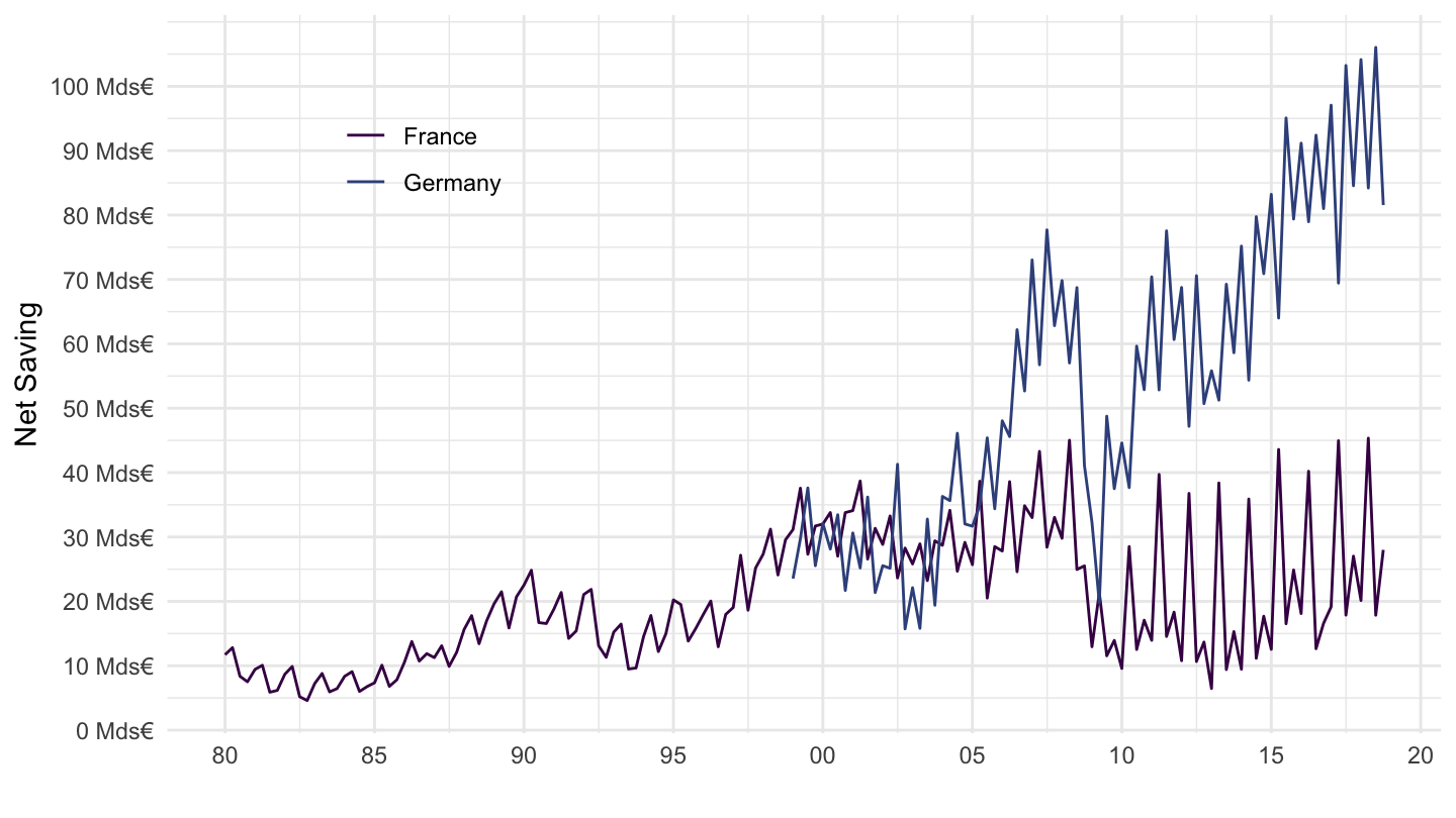
Example 4: Europe VS U.S. since Global Financial Crisis
Code
QNA_ARCHIVE %>%
  filter(SUBJECT == "B1_GE",
         MEASURE == "VOBARSA",
         FREQUENCY == "Q",
         LOCATION %in% c("EA19", "USA")) %>%
  quarter_to_date %>%
  filter(date >= as.Date("2000-01-01")) %>%
  left_join(QNA_ARCHIVE_var$LOCATION %>% rename(LOCATION = id), by = "LOCATION") %>%
  group_by(LOCATION) %>%
  arrange(date) %>%
  mutate(obsValue = 100 * obsValue / obsValue[date == as.Date("2007-01-01")]) %>%
  ggplot(.) + geom_line(aes(x = date, y = obsValue, color = label, linetype = label)) +
  scale_color_manual(values = viridis(3)[1:2]) +
  theme_minimal() + xlab("") + ylab("") +
  geom_rect(data = nber_recessions,
            aes(xmin = Peak, xmax = Trough, ymin = 0, ymax = +Inf),
            fill = 'grey', alpha = 0.5) +
  scale_x_date(breaks = seq(1960, 2020, 1) %>% paste0("-01-01") %>% as.Date,
               labels = date_format("%y"),
               limits = c(2000, 2019) %>% paste0("-01-01") %>% as.Date) +
  theme(legend.position = c(0.2, 0.85),
        legend.title = element_blank()) +
  scale_y_log10(breaks = seq(70, 200, 5))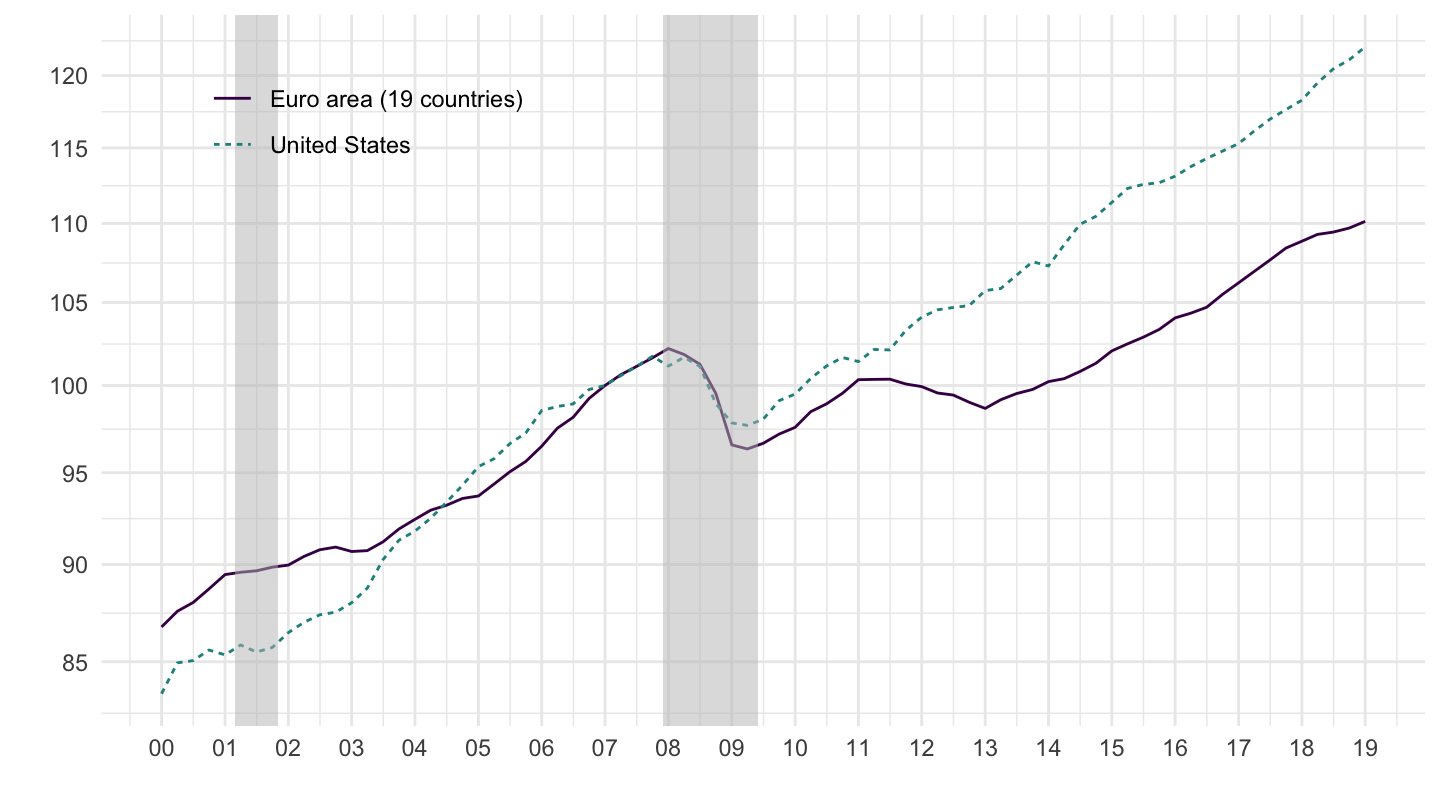
Example 5: European Heterogeneity since the GFC
Code
QNA_ARCHIVE %>%
  filter(SUBJECT == "B1_GE",
         MEASURE == "VOBARSA",
         FREQUENCY == "Q",
         LOCATION %in% c("ITA", "DEU", "GRC", "ESP", "PRT", "FRA")) %>%
  quarter_to_date %>%
  filter(date >= as.Date("2000-01-01")) %>%
  left_join(QNA_ARCHIVE_var$LOCATION %>% rename(LOCATION = id), by = "LOCATION") %>%
  group_by(LOCATION) %>%
  arrange(date) %>%
  mutate(obsValue = 100 * obsValue / obsValue[date == as.Date("2007-01-01")]) %>%
  ggplot(.) + geom_line(aes(x = date, y = obsValue, color = label, linetype = label)) +
  scale_color_manual(values = viridis(7)[1:6]) +
  theme_minimal() + xlab("") + ylab("") +
  geom_rect(data = nber_recessions,
            aes(xmin = Peak, xmax = Trough, ymin = 0, ymax = +Inf),
            fill = 'grey', alpha = 0.5) +
  scale_x_date(breaks = seq(1960, 2020, 1) %>% paste0("-01-01") %>% as.Date,
               labels = date_format("%y"),
               limits = c(2000, 2019) %>% paste0("-01-01") %>% as.Date) +
  theme(legend.position = c(0.25, 0.9),
        legend.title = element_blank(),
        legend.direction = "horizontal") +
  scale_y_log10(breaks = seq(70, 200, 5))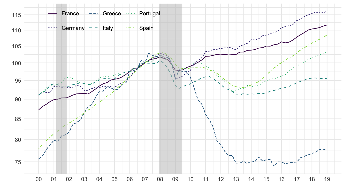
Example 6: Exports and Imports in Japan (Value)
(ref:JPN-X-M-GDP) Exports and Imports, Japan (percentage of GDP)
Code
QNA_ARCHIVE %>%
  filter(SUBJECT %in% c("P6", "P7", "B1_GE"),
         MEASURE == "VOBARSA",
         FREQUENCY == "Q",
         LOCATION == "JPN") %>%
  quarter_to_date %>%
  mutate(variable = paste0(SUBJECT, "_", MEASURE)) %>%
  select(date, variable, obsValue) %>%
  spread(variable, obsValue) %>%
  mutate(`Exports (% of GDP)` = P6_VOBARSA / B1_GE_VOBARSA,
         `Imports (% of GDP)` = P7_VOBARSA / B1_GE_VOBARSA) %>%
  na.omit %>%
  select(-contains("VOBARSA")) %>%
  gather(variable, value, - date) %>%
  ggplot() + geom_line(aes(x = date, y = value, color = variable, linetype = variable)) +
  scale_color_manual(values = viridis(4)[1:3]) +
  theme_minimal() +
  scale_x_date(breaks = seq(1920, 2025, 5) %>% paste0("-01-01") %>% as.Date,
               labels = date_format("%y")) +
  theme(legend.position = c(0.45, 0.9),
        legend.title = element_blank()) +
  scale_y_continuous(breaks = 0.01*seq(0, 60, 5),
                     labels = scales::percent_format(accuracy = 1)) +
  ylab("% of GDP (Japan)") + xlab("")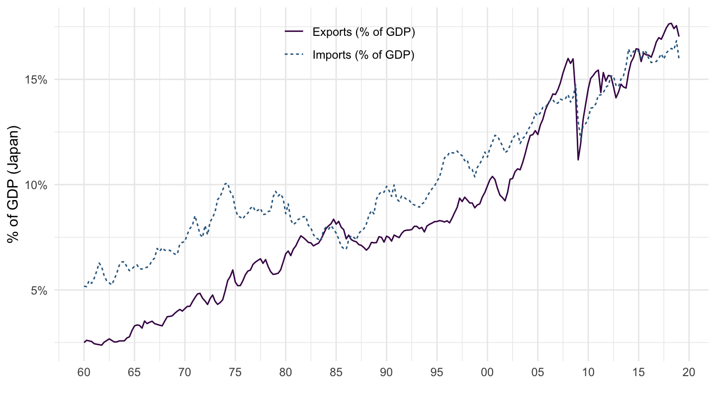
Example 7: Japan’s CA = S-I
Code
QNA_ARCHIVE %>%
  filter(SUBJECT %in% c("P6", "P7", "P51", "B1_GE"),
         MEASURE == "VOBARSA",
         FREQUENCY == "Q",
         LOCATION == "FRA") %>%
  quarter_to_date %>%
  mutate(variable = paste0(SUBJECT, "_", MEASURE)) %>%
  select(date, variable, obsValue) %>%
  spread(variable, obsValue) %>%
  mutate(`Saving (% of GDP)` = (P6_VOBARSA - P7_VOBARSA + P51_VOBARSA) / B1_GE_VOBARSA,
         `Investment (% of GDP)` = P51_VOBARSA / B1_GE_VOBARSA) %>%
  na.omit %>%
  select(-contains("VOBARSA")) %>%
  gather(variable, value, - date) %>%
  ggplot() + geom_line(aes(x = date, y = value, color = variable, linetype = variable)) +
  scale_color_manual(values = viridis(4)[1:3]) +
  theme_minimal() +
  scale_x_date(breaks = seq(1920, 2025, 5) %>% paste0("-01-01") %>% as.Date,
               labels = date_format("%y")) +
  theme(legend.position = c(0.45, 0.9),
        legend.title = element_blank()) +
  scale_y_continuous(breaks = 0.01*seq(-7, 60, 1),
                     labels = scales::percent_format(accuracy = 1)) +
  ylab("% of GDP") + xlab("")