Monthly unemployment rates - IALFS_UNE_M

Data - OECD

Last observation: Q2 2026 (N = 772) · août 2026 (N = 36) · 2025 (N = 752)

First observation: 1953 (N = 4) · janv. 1953 (N = 4) · Q1 1953 (N = 4)

Last data update: 14 sept. 2026, 23:27

Last compile: 14 sept. 2026, 23:45

Structure

REF_AREA

MEASURE

UNIT_MEASURE

TRANSFORMATION

ADJUSTMENT

SEX

AGE

ACTIVITY

FREQ

Unemployment rate

IALFS_UNE_M is the OECD’s harmonised monthly unemployment rate (unemployed as a share of the labour force), seasonally adjusted, for ~40 countries plus the Euro area, EU, G7 and OECD aggregates. Rates are available by sex and for three age groups (15+, 25+, and 15–24). Grey bands mark US (NBER) recessions.

United States, Euro area, France, Germany, Italy, Spain - since 1999

une_m(c("USA", "EA", "FRA", "DEU", "ESP", "ITA"), from = "1999-01-01") |>
  add_flag_color("Ref_area") |>
  line_flags(recessions = TRUE)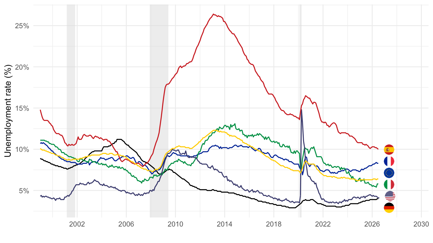

United States vs. Euro area - the long run, since 1990

une_m(c("USA", "EA"), from = "1990-01-01") |>
  add_flag_color("Ref_area") |>
  line_flags(recessions = TRUE, xby = 3)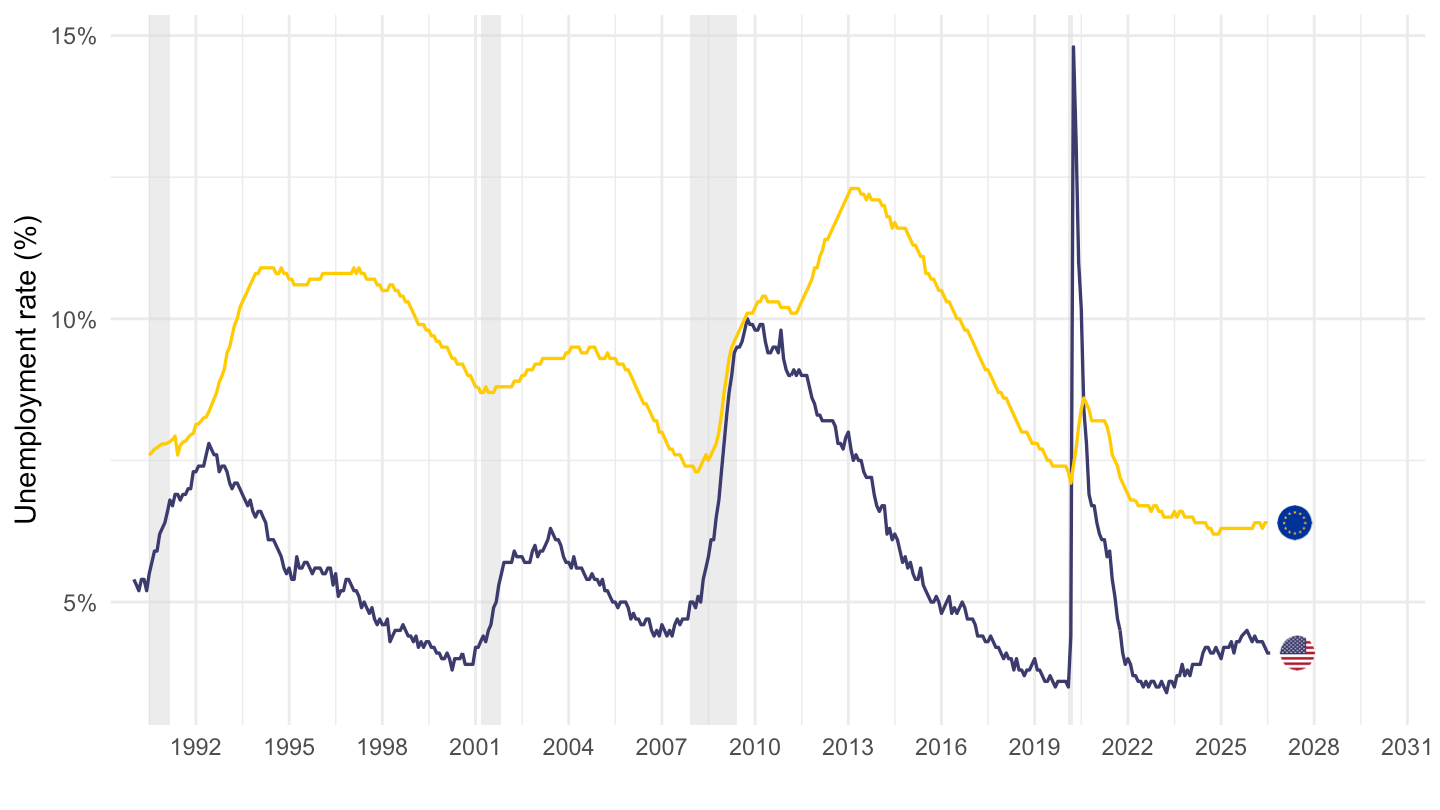

United States, Japan, Canada - since 1955

Japan and the United States are the two countries with the longest monthly series (from 1955).

une_m(c("USA", "JPN", "CAN"), from = "1955-01-01") |>
  add_flag_color("Ref_area") |>
  line_flags(recessions = TRUE, xby = 10, yby = 2)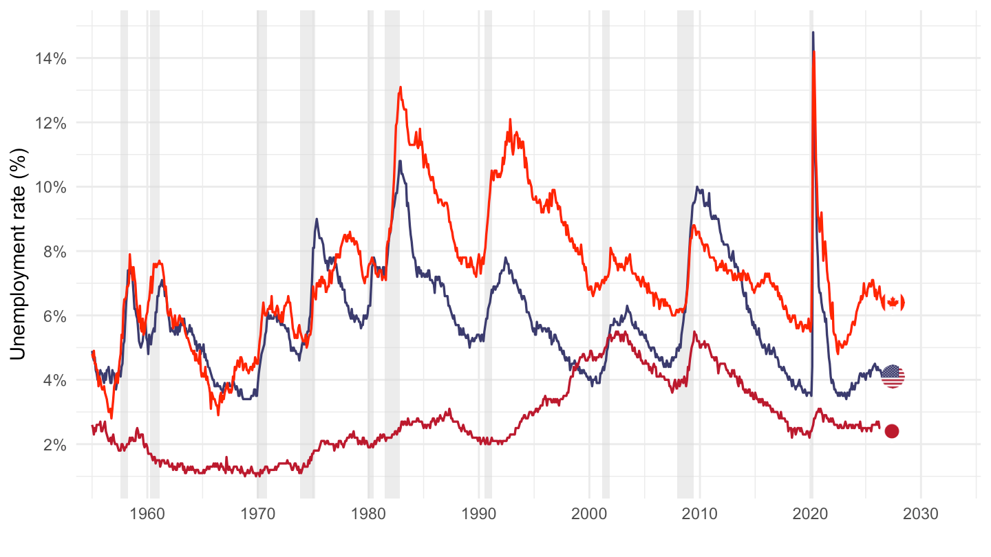

English-speaking economies - since 1983

une_m(c("USA", "GBR", "CAN", "AUS", "NZL"), from = "1983-01-01") |>
  add_flag_color("Ref_area") |>
  line_flags(xby = 5, yby = 2)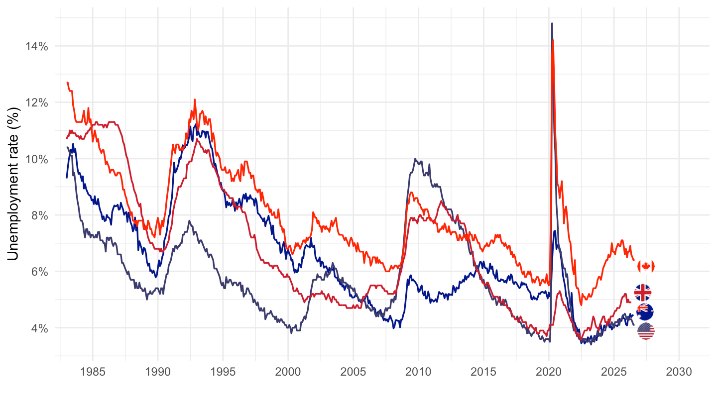

Southern Europe - since 2000

une_m(c("ESP", "GRC", "ITA", "PRT", "FRA", "EA"), from = "2000-01-01") |>
  add_flag_color("Ref_area") |>
  line_flags(recessions = TRUE)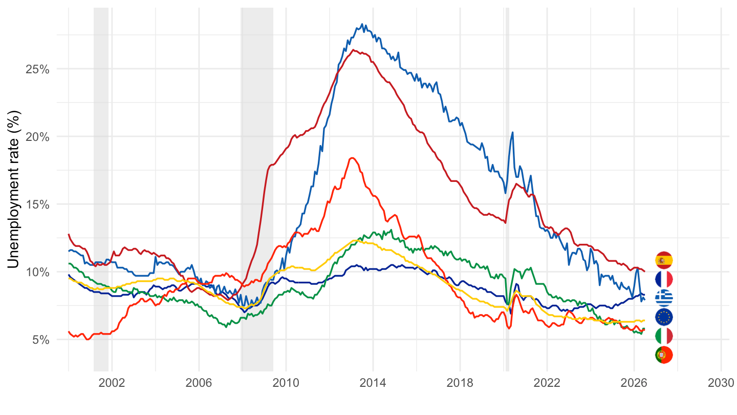

Central & Eastern Europe - since 2000

une_m(c("POL", "CZE", "HUN", "SVK", "ROU", "HRV"), from = "2000-01-01") |>
  add_flag_color("Ref_area") |>
  line_flags(yby = 2)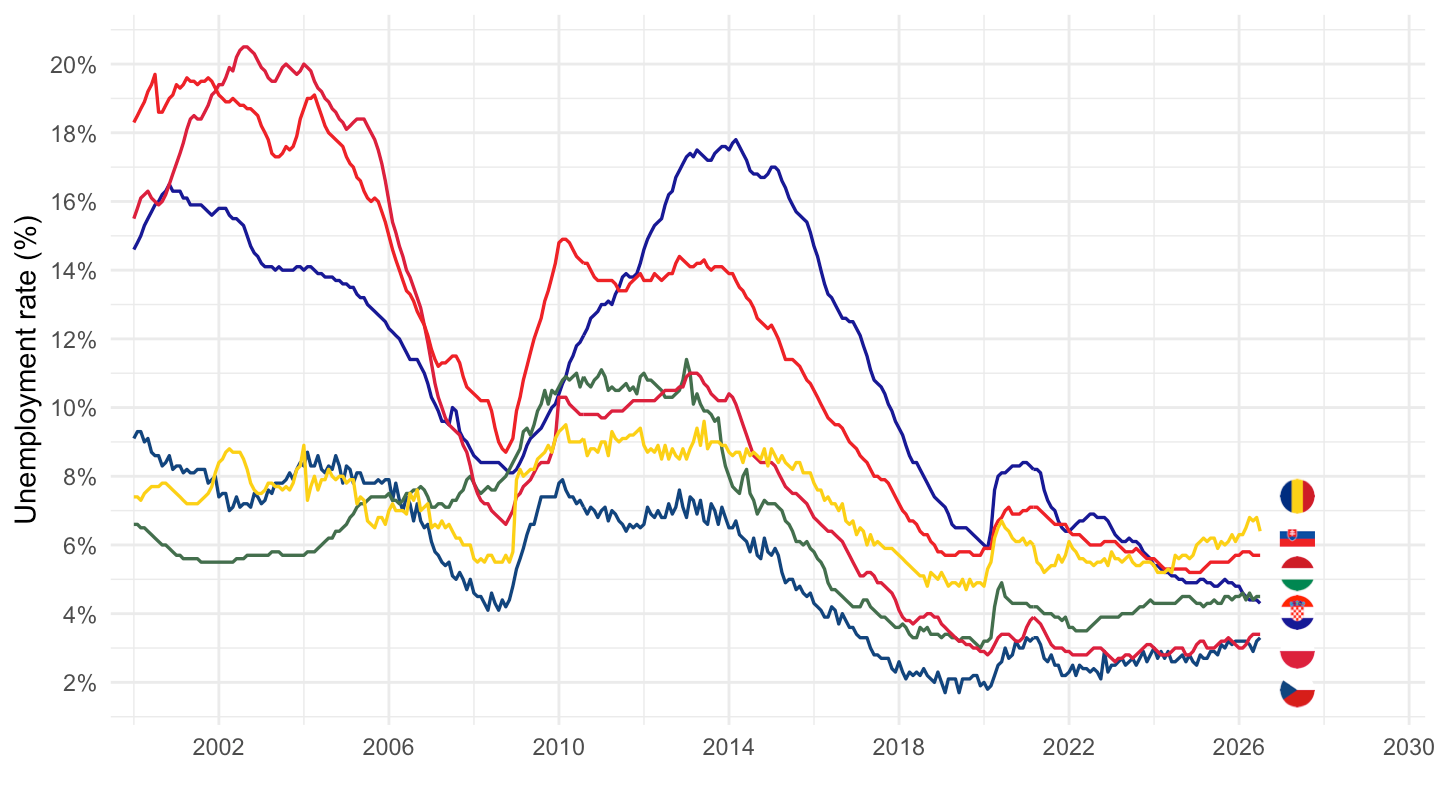

Nordic countries - since 1990

une_m(c("SWE", "FIN", "NOR", "DNK", "DEU"), from = "1990-01-01") |>
  add_flag_color("Ref_area") |>
  line_flags(yby = 2)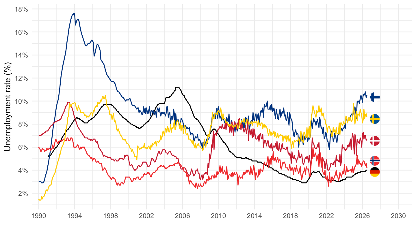

Aggregates: OECD, G7, Euro area, EU, United States - since 2001

The OECD area carries the OECD emblem (icon/flag/round/oecd.png); G7 has no round icon and is labelled at its line end.

d <- une_m(c("OECD", "G7", "EA", "EU", "USA"), from = "2001-01-01") |>
  add_flag_color("Ref_area") |>
  mutate(color = ifelse(Ref_area == "G7", "grey35", color))   # G7 has no flag -> neutral grey
line_flags(d, xby = 3, yby = 2) +
  geom_text(
    data = function(df) { g <- df[df$Ref_area == "G7", ]; g[g$date == max(g$date), ] },
    aes(label = "G7"), hjust = -0.35, vjust = 0.4, size = 2.6, color = "grey35")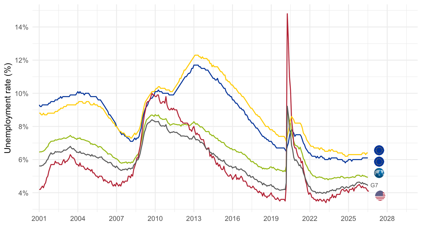

Youth unemployment (15–24)

Youth unemployment rates run 2–3× the headline rate and peaked above 55% in Spain and Greece after the euro crisis.

Spain, Greece, Italy, France, Germany, US

une_m(c("ESP", "GRC", "ITA", "FRA", "DEU", "USA"), age = "Y15T24",
      from = "2000-01-01") |>
  add_flag_color("Ref_area") |>
  line_flags(ylab = "Youth (15–24) unemployment rate (%)", yby = 10)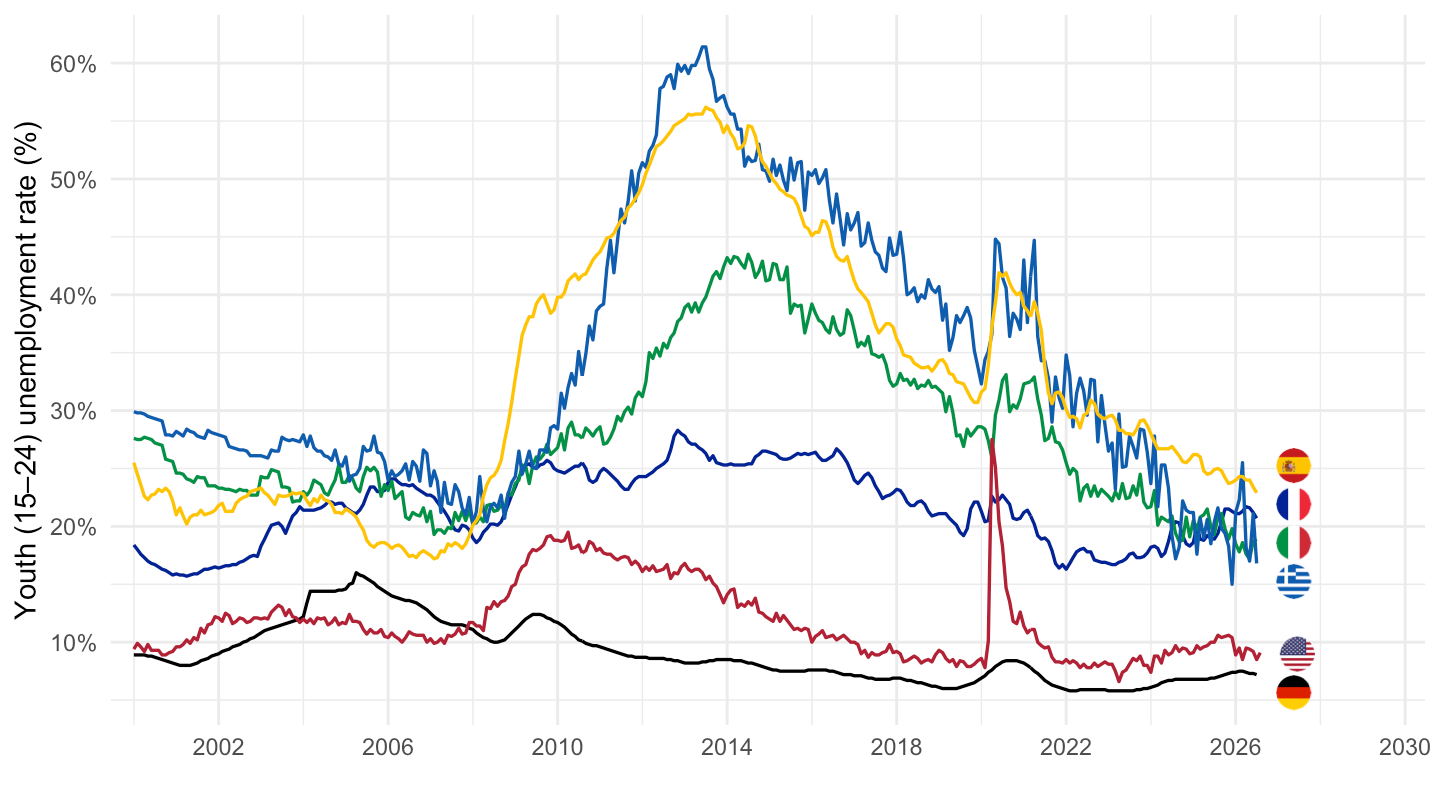

Europe, US, OECD

une_m(c("EA", "USA", "OECD"), age = "Y15T24",
      from = "2000-01-01") |>
  add_flag_color("Ref_area") |>
  line_flags(ylab = "Youth (15–24) unemployment rate (%)", yby = 5, xby = 2)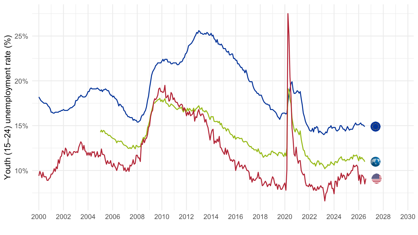

Europe, US, OECD, France

une_m(c("EA", "USA", "OECD"), age = "Y15T24",
      from = "2000-01-01") |>
  add_flag_color("Ref_area") |>
  line_flags(ylab = "Youth (15–24) unemployment rate (%)", yby = 5, xby = 2)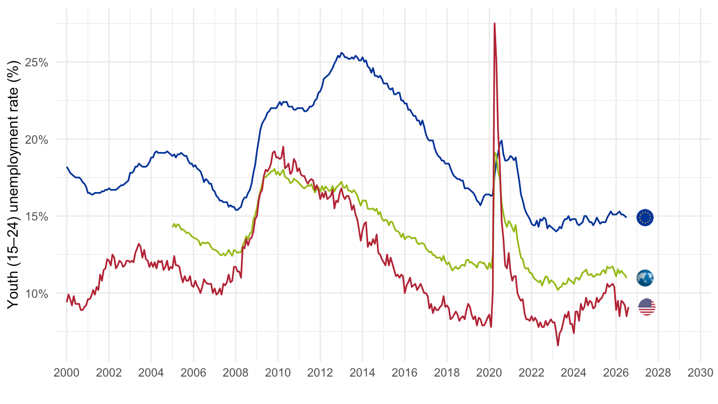

Youth unemployment today, ranked

youth_now <- IALFS_UNE_M |>
  filter(FREQ == "M", SEX == "_T", ADJUSTMENT == "Y", AGE == "Y15T24",
         !REF_AREA %in% c("EA", "EU", "OECD", "G7")) |>
  month_to_date() |>
  filter(!is.na(obsValue)) |>
  group_by(REF_AREA, Ref_area) |>
  filter(date == max(date)) |>
  ungroup() |>
  mutate(Ref_area = area_relabel(Ref_area)) |>
  add_flag_color("Ref_area") |>
  mutate(color = ifelse(is.na(color) | toupper(color) %in% c("#FFFFFF", "#FEFEFE"),
                        "grey60", color)) |>
  arrange(obsValue) |>
  mutate(Ref_area = factor(Ref_area, levels = Ref_area))

ggplot(youth_now, aes(obsValue, Ref_area, fill = color)) +
  geom_col(width = 0.7, color = "grey35", linewidth = 0.15) +
  geom_text(aes(label = paste0(round(obsValue, 1), "%")), hjust = -0.15, size = 2.6) +
  scale_fill_identity() +
  scale_x_continuous(expand = expansion(mult = c(0, 0.1))) +
  theme_minimal() + theme(panel.grid.major.y = element_blank()) +
  xlab("Youth unemployment rate (%), latest month") + ylab("")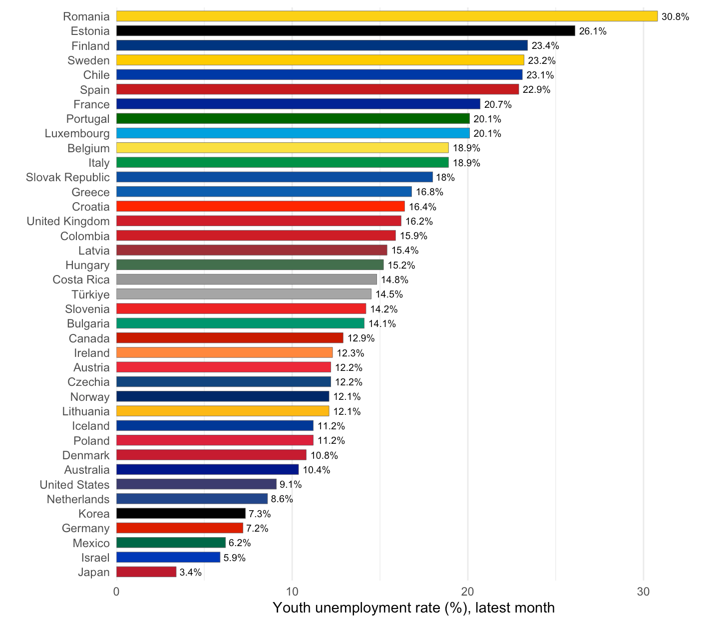

Men and women

IALFS_UNE_M |>
  filter(REF_AREA %in% c("USA", "EA", "FRA", "DEU", "ITA", "ESP"),
         FREQ == "M", SEX %in% c("M", "F"), ADJUSTMENT == "Y", AGE == "Y_GE15") |>
  month_to_date() |>
  mutate(Ref_area = area_relabel(Ref_area)) |>
  filter(date >= as.Date("2000-01-01"), !is.na(obsValue)) |>
  ggplot(aes(date, obsValue, color = Sex)) +
  geom_line(linewidth = 0.5) +
  facet_wrap(~ Ref_area) +
  scale_color_manual(values = c("Female" = "#C1447E", "Male" = "#3B7DB3"), name = NULL) +
  theme_minimal() + theme(legend.position = "bottom") +
  xlab("") + ylab("Unemployment rate (%)") +
  x_years(8) + y_pct(5)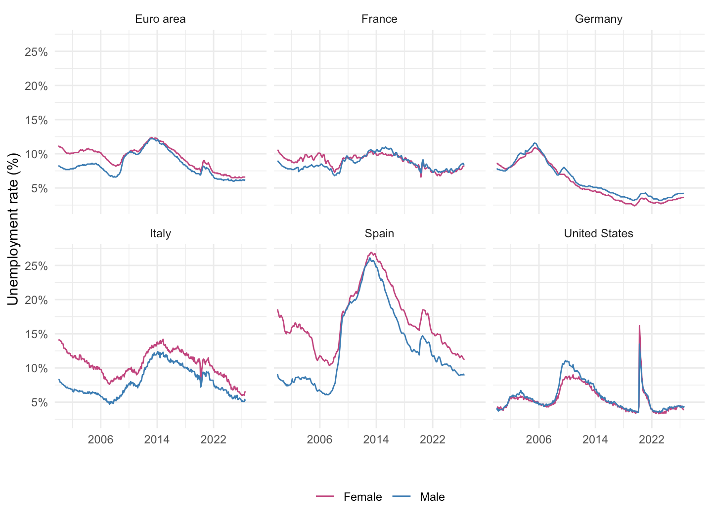

Where unemployment stands today

Latest available month for each country (seasonally adjusted, 15+).

now <- IALFS_UNE_M |>
  filter(FREQ == "M", SEX == "_T", ADJUSTMENT == "Y", AGE == "Y_GE15",
         !REF_AREA %in% c("EA", "EU", "OECD", "G7")) |>
  month_to_date() |>
  filter(!is.na(obsValue)) |>
  group_by(REF_AREA, Ref_area) |>
  filter(date == max(date)) |>
  ungroup() |>
  mutate(Ref_area = area_relabel(Ref_area)) |>
  add_flag_color("Ref_area") |>
  mutate(color = ifelse(is.na(color) | toupper(color) %in% c("#FFFFFF", "#FEFEFE"),
                        "grey60", color)) |>
  arrange(obsValue) |>
  mutate(Ref_area = factor(Ref_area, levels = Ref_area))

ggplot(now, aes(obsValue, Ref_area, fill = color)) +
  geom_col(width = 0.7, color = "grey35", linewidth = 0.15) +
  geom_text(aes(label = paste0(round(obsValue, 1), "%")), hjust = -0.15, size = 2.6) +
  scale_fill_identity() +
  scale_x_continuous(expand = expansion(mult = c(0, 0.1))) +
  theme_minimal() + theme(panel.grid.major.y = element_blank()) +
  xlab("Unemployment rate (%), latest month") + ylab("")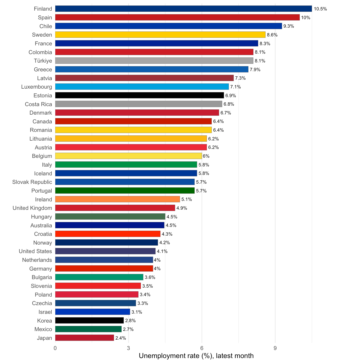

Change since just before COVID (January 2020)

base <- IALFS_UNE_M |>
  filter(FREQ == "M", SEX == "_T", ADJUSTMENT == "Y", AGE == "Y_GE15",
         obsTime == "2020-01", !REF_AREA %in% c("EA", "EU", "OECD", "G7")) |>
  transmute(REF_AREA, Ref_area = area_relabel(Ref_area), pre = obsValue)

covid <- now |>
  select(REF_AREA, cur = obsValue) |>
  inner_join(base, by = "REF_AREA") |>
  mutate(chg = cur - pre) |>
  arrange(chg) |>
  mutate(Ref_area = factor(Ref_area, levels = Ref_area))

ggplot(covid, aes(y = Ref_area)) +
  geom_segment(aes(x = pre, xend = cur, yend = Ref_area), color = "grey70") +
  geom_point(aes(x = pre), color = "grey55", size = 2) +
  geom_point(aes(x = cur, color = chg > 0), size = 2.4) +
  scale_color_manual(values = c(`TRUE` = "#C0392B", `FALSE` = "#2E8B57"),
                     labels = c(`TRUE` = "higher than 2020", `FALSE` = "lower than 2020"),
                     name = NULL) +
  theme_minimal() + theme(legend.position = "bottom",
                          panel.grid.major.y = element_blank()) +
  xlab("Unemployment rate (%): grey = Jan 2020, coloured = latest") + ylab("")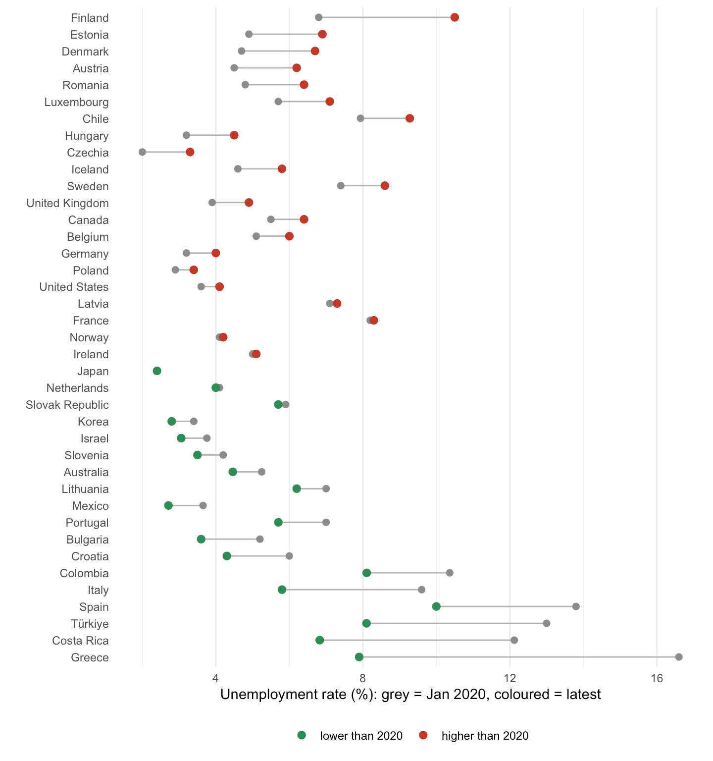

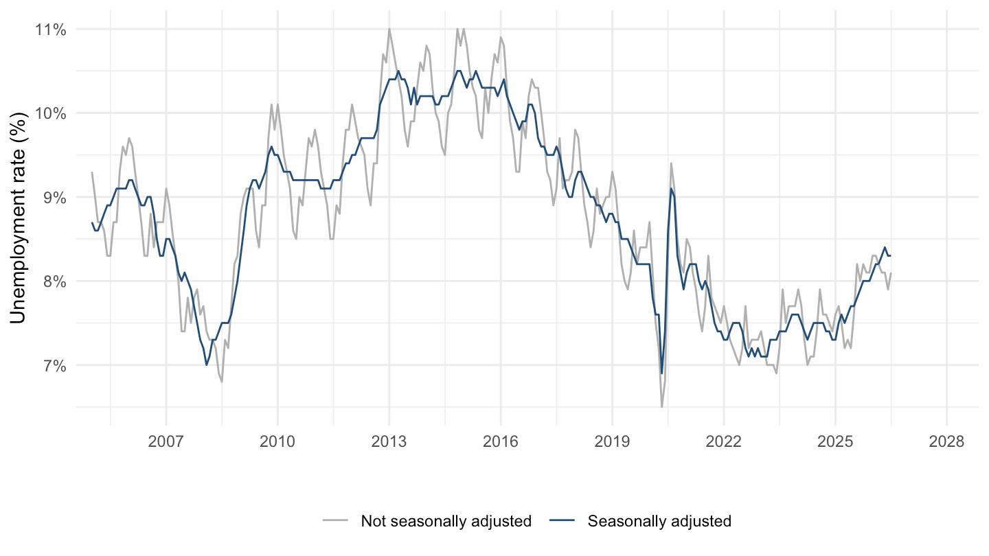
Seasonal adjustment

Raw (not seasonally adjusted) vs. seasonally adjusted rate, France.

IALFS_UNE_M |>
  filter(REF_AREA == "FRA", FREQ == "M", SEX == "_T", AGE == "Y_GE15") |>
  month_to_date() |>
  filter(date >= as.Date("2005-01-01"), !is.na(obsValue)) |>
  mutate(adj = ifelse(ADJUSTMENT == "Y", "Seasonally adjusted",
                      "Not seasonally adjusted")) |>
  ggplot(aes(date, obsValue, color = adj)) +
  geom_line(linewidth = 0.5) +
  scale_color_manual(values = c("Not seasonally adjusted" = "#B0B0B0",
                                "Seasonally adjusted" = "#1F4E79"), name = NULL) +
  theme_minimal() + theme(legend.position = "bottom") +
  xlab("") + ylab("Unemployment rate (%)") +
  x_years(3) + y_pct(1)