GENDER_EMP %>%
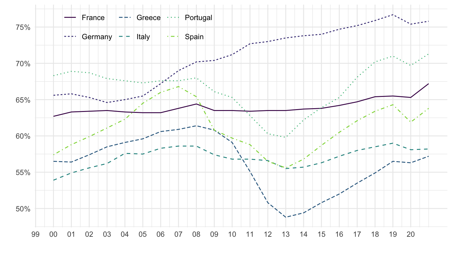
filter(IND == "EMP2",
SEX == "ALL_PERSONS",
AGE == "1564",
COU %in% c("ITA", "DEU", "GRC", "ESP", "PRT", "FRA")) %>%
arrange(COU, TIME) %>%
rename(obsTime = TIME) %>%
year_to_date %>%
filter(date >= as.Date("2000-01-01")) %>%
left_join(GENDER_EMP_var$COU %>%
setNames(c("COU", "Cou")), by = "COU") %>%
group_by(COU) %>%
arrange(date) %>%
ggplot(.) + geom_line(aes(x = date, y = obsValue/100, color = Cou, linetype = Cou)) +
scale_color_manual(values = viridis(7)[1:6]) +
theme_minimal() + xlab("") + ylab("") +
scale_x_date(breaks = seq(1960, 2020, 1) %>% paste0("-01-01") %>% as.Date,
labels = date_format("%y")) +
theme(legend.position = c(0.25, 0.9),
legend.title = element_blank(),
legend.direction = "horizontal") +
scale_y_continuous(breaks = 0.01*seq(0, 200, 5),
labels = scales::percent_format(accuracy = 1))