Economic Outlook, Wage - EO_WAGE

Data - OECD

Author

Info

LAST_DOWNLOAD

LAST_DOWNLOAD
2022-10-04

LAST_COMPILE

LAST_COMPILE
2026-07-26

Last

obsTime	Nobs
2023-Q4	22

FREQUENCY

Code

EO %>%
  left_join(EO_var$FREQUENCY, by = "FREQUENCY") %>%
  group_by(FREQUENCY, Frequency) %>%
  summarise(Nobs = n()) %>%
  arrange(-Nobs) %>%
  print_table_conditional()

FREQUENCY	Frequency	Nobs
Q	Quarterly	4396
A	Annual	1494

LOCATION

Code

EO %>%
  left_join(EO_var$LOCATION, by = "LOCATION") %>%
  group_by(LOCATION, Location) %>%
  summarise(Nobs = n()) %>%
  arrange(-Nobs) %>%
  mutate(Flag = gsub(" ", "-", str_to_lower(Location)),
         Flag = paste0('<img src="../../icon/flag/vsmall/', Flag, '.png" alt="Flag">')) %>%
  select(Flag, everything()) %>%
  {if (is_html_output()) datatable(., filter = 'top', rownames = F, escape = F) else .}

France, Germany, Italy

All

Code

EO %>%
  filter(LOCATION %in% c("FRA", "DEU", "ITA")) %>%
  left_join(EO_var$LOCATION, by = "LOCATION") %>%
  year_to_date %>%
  mutate(obsValue = obsValue/10^9) %>%
  ggplot() + theme_minimal() + ylab("Wages") + xlab("") +
  geom_line(aes(x = date, y = obsValue, color = Location)) + add_3flags +
  scale_color_manual(values = c("#0055a4", "#000000", "#008c45")) +
  scale_x_date(breaks = seq(1920, 2100, 5) %>% paste0("-01-01") %>% as.Date,
               labels = date_format("%Y")) +
  theme(legend.position = c(0.15, 0.2),
        legend.title = element_blank()) +
  scale_y_log10(breaks = c(1, 2, 3, 5, 10, 20, 30, 50, 80,
                           100, 200, 300, 500, 1000, 2000))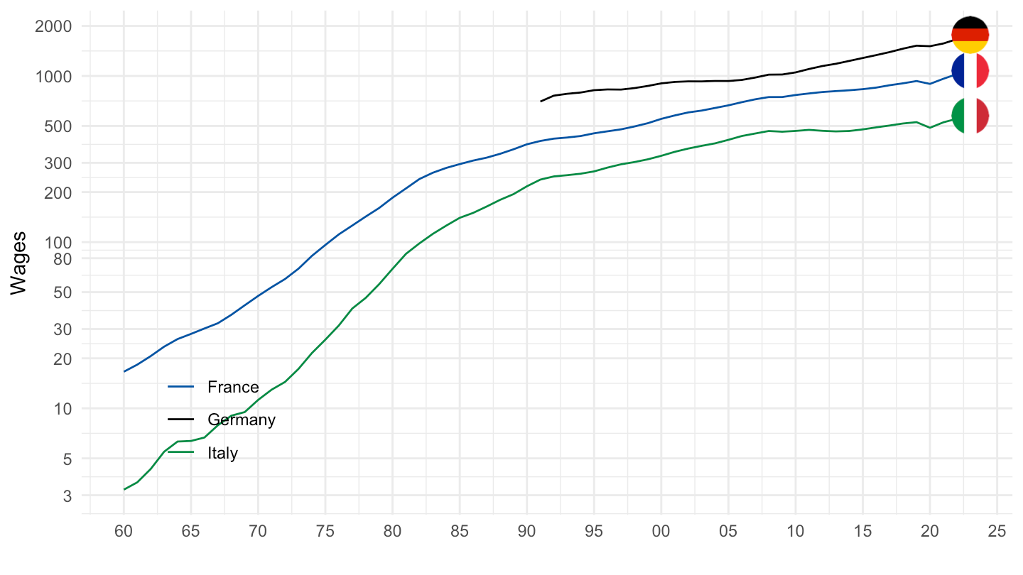

1995-

Annual

Code

EO %>%
  filter(LOCATION %in% c("FRA", "DEU", "ITA"),
         FREQUENCY == "A") %>%
  left_join(EO_var$LOCATION, by = "LOCATION") %>%
  year_to_date %>%
  filter(date >= as.Date("1995-01-01")) %>%
  mutate(obsValue = obsValue/10^9) %>%
  ggplot() + theme_minimal() + ylab("Wages") + xlab("") +
  geom_line(aes(x = date, y = obsValue, color = Location)) + add_3flags +
  scale_color_manual(values = c("#0055a4", "#000000", "#008c45")) +
  scale_x_date(breaks = seq(1920, 2100, 5) %>% paste0("-01-01") %>% as.Date,
               labels = date_format("%Y")) +
  theme(legend.position = c(0.15, 0.2),
        legend.title = element_blank()) +
  scale_y_log10(breaks = c(1, 2, 3, 5, 10, 20, 30, 50, 80,
                           100, 200, 300, 500, 1000, 2000))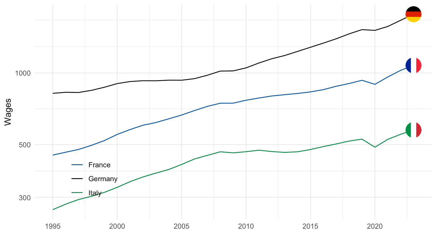

Quarterly

Code

EO %>%
  filter(LOCATION %in% c("FRA", "DEU", "ITA"),
         FREQUENCY == "Q") %>%
  left_join(EO_var$LOCATION, by = "LOCATION") %>%
  quarter_to_date %>%
  filter(date >= as.Date("1995-01-01")) %>%
  mutate(obsValue = obsValue/10^9) %>%
  ggplot() + theme_minimal() + ylab("Wages") + xlab("") +
  geom_line(aes(x = date, y = obsValue, color = Location)) + add_3flags +
  scale_color_manual(values = c("#0055a4", "#000000", "#008c45")) +
  scale_x_date(breaks = seq(1920, 2100, 5) %>% paste0("-01-01") %>% as.Date,
               labels = date_format("%Y")) +
  theme(legend.position = c(0.15, 0.2),
        legend.title = element_blank()) +
  scale_y_log10(breaks = c(1, 2, 3, 5, 10, 20, 30, 50, 80,
                           100, 200, 300, 500, 1000, 2000))