Last observation: Q4 2025 (N = 4171) · 2025 (N = 9269)
First observation: 1960 (N = 1651) · Q1 1960 (N = 1215)
Last data update: 02 août 2026, 08:58
Last compile: 05 oct. 2026, 00:25
NULL
EO_115_extract <- EO_115 |>
  filter(FREQ == "Q",
         REF_AREA == "DEU",
         MEASURE == "GDPV") |>
select(obsTime, obsValue)EO_116_extract <- EO_116 |>
filter(FREQ == "Q",
REF_AREA == "DEU",
MEASURE == "GDPV") |>
select(obsTime, obsValue)EO_117_extract <- EO_117 |>
filter(FREQ == "Q",
REF_AREA == "DEU",
MEASURE == "GDPV") |>
select(obsTime, obsValue)EO110_INTERNET |>
mutate(vintage = "Economic Outlook No 110 - December 2021") |>
bind_rows(EO111_INTERNET |>
mutate(vintage = "Economic Outlook No 111 - June 2022")) |>
bind_rows(EO112_INTERNET |>
mutate(vintage = "Economic Outlook No 112 - November 2022")) |>
bind_rows(EO114_INTERNET |>
mutate(vintage = "Economic Outlook No 113 - June 2023")) |>
bind_rows(EO114_INTERNET |>
mutate(vintage = "Economic Outlook No 114 - November 2023")) |>
filter(VARIABLE == "GDPV",
LOCATION == "DEU",
FREQUENCY == "Q") |>
bind_rows(EO_115_extract) |>
bind_rows(EO_116_extract) |>
bind_rows(EO_117_extract) |>
quarter_to_date() |>
filter(date >= as.Date("2007-01-01")) |>
group_by(vintage) |>
mutate(obsValue = 100*obsValue/obsValue[date == as.Date("2007-01-01")]) |>
ggplot() + geom_line(aes(x = date, y = obsValue, color = vintage)) +
xlab("") + ylab("Gross Domestic Product in Volume, Germany") + theme_minimal() +
scale_x_date(breaks = seq(1920, 2100, 1) |> paste0("-01-01") |> as.Date(),
labels = date_format("%Y")) +
theme(legend.position = c(0.25, 0.9),
legend.title = element_blank()) +
scale_y_log10(breaks = seq(20, 200, 1))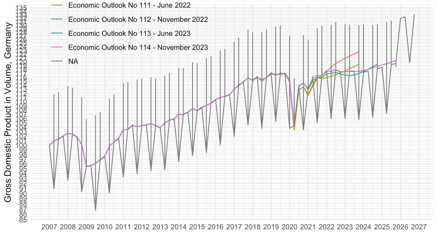
EO110_INTERNET |>
  mutate(vintage = "Economic Outlook No 110 - December 2021") |>
  bind_rows(EO111_INTERNET |>
              mutate(vintage = "Economic Outlook No 111 - June 2022")) |>
  bind_rows(EO112_INTERNET |>
              mutate(vintage = "Economic Outlook No 112 - November 2022")) |>
  bind_rows(EO114_INTERNET |>
              mutate(vintage = "Economic Outlook No 113 - June 2023")) |>
  bind_rows(EO114_INTERNET |>
              mutate(vintage = "Economic Outlook No 114 - November 2023")) |>
  filter(VARIABLE == "GDPV",
         LOCATION == "DEU",
         FREQUENCY == "Q") |>
  bind_rows(EO_115_extract) |>
  bind_rows(EO_116_extract) |>
  bind_rows(EO_117_extract) |>
  quarter_to_date() |>
  filter(date >= as.Date("2014-01-01")) |>
  group_by(vintage) |>
  mutate(obsValue = 100*obsValue/obsValue[date == as.Date("2014-01-01")]) |>
  ggplot() + geom_line(aes(x = date, y = obsValue, color = vintage)) +
  xlab("") + ylab("Gross Domestic Product in Volume, Germany") + theme_minimal() +
  scale_x_date(breaks = seq(1920, 2100, 1) |> paste0("-01-01") |> as.Date(),
               labels = date_format("%Y")) +
  theme(legend.position = c(0.25, 0.9),
        legend.title = element_blank()) +
  scale_y_log10(breaks = seq(20, 200, 1))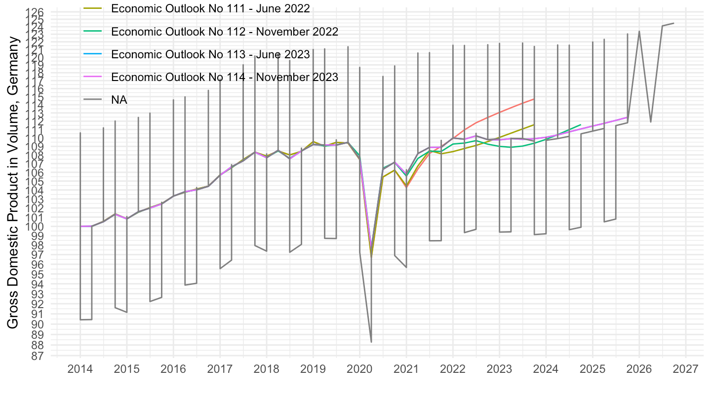
EO110_INTERNET |>
  mutate(vintage = "Economic Outlook No 110 - December 2021") |>
  bind_rows(EO111_INTERNET |>
              mutate(vintage = "Economic Outlook No 111 - June 2022")) |>
  bind_rows(EO112_INTERNET |>
              mutate(vintage = "Economic Outlook No 112 - November 2022")) |>
  bind_rows(EO113_INTERNET |>
              mutate(vintage = "Economic Outlook No 113 - June 2023")) |>
  bind_rows(EO114_INTERNET |>
              mutate(vintage = "Economic Outlook No 114 - November 2023")) |>
  filter(VARIABLE == "GDPV",
         LOCATION == "DEU",
         FREQUENCY == "Q") |>
  bind_rows(EO_115_extract) |>
  bind_rows(EO_116_extract) |>
  bind_rows(EO_117_extract) |>
  quarter_to_date() |>
  filter(date >= as.Date("2017-01-01")) |>
  group_by(vintage) |>
  mutate(obsValue = 100*obsValue/obsValue[date == as.Date("2017-01-01")]) |>
  ggplot() + geom_line(aes(x = date, y = obsValue, color = vintage)) +
  xlab("") + ylab("Gross Domestic Product in Volume, Germany") + theme_minimal() +
  scale_x_date(breaks = seq(1920, 2100, 1) |> paste0("-01-01") |> as.Date(),
               labels = date_format("%Y")) +
  theme(legend.position = c(0.7, 0.2),
        legend.title = element_blank()) +
  scale_y_log10(breaks = seq(20, 200, 1))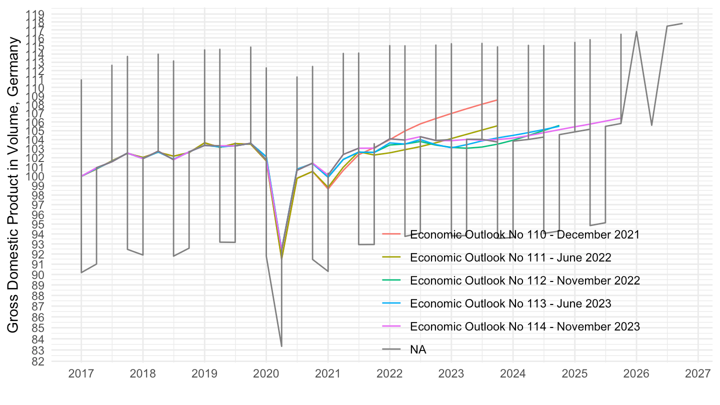
EO110_INTERNET |>
  mutate(vintage = "Economic Outlook No 110 - December 2021") |>
  bind_rows(EO111_INTERNET |>
              mutate(vintage = "Economic Outlook No 111 - June 2022")) |>
  bind_rows(EO112_INTERNET |>
              mutate(vintage = "Economic Outlook No 112 - November 2022")) |>
  bind_rows(EO113_INTERNET |>
              mutate(vintage = "Economic Outlook No 113 - June 2023")) |>
  bind_rows(EO114_INTERNET |>
              mutate(vintage = "Economic Outlook No 114 - November 2023")) |>
  filter(VARIABLE == "GDPV",
         LOCATION == "DEU",
         FREQUENCY == "Q") |>
  bind_rows(EO_115_extract) |>
  bind_rows(EO_116_extract) |>
  bind_rows(EO_117_extract) |>
  quarter_to_date() |>
  filter(date >= as.Date("2019-10-01")) |>
  group_by(vintage) |>
  mutate(obsValue = 100*obsValue/obsValue[date == as.Date("2019-10-01")]) |>
  ggplot() + geom_line(aes(x = date, y = obsValue, color = vintage)) +
  xlab("") + ylab("Gross Domestic Product in Volume, Germany") + theme_minimal() +
  scale_x_date(breaks = seq(1920, 2100, 1) |> paste0("-01-01") |> as.Date(),
               labels = date_format("%Y")) +
  theme(legend.position = c(0.7, 0.2),
        legend.title = element_blank()) +
  scale_y_log10(breaks = seq(20, 200, 1))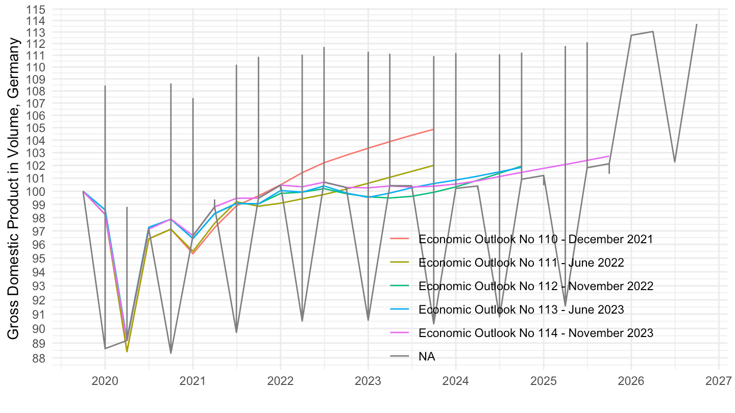
EO110_INTERNET |>
  mutate(vintage = "Economic Outlook No 110 - December 2021") |>
  bind_rows(EO111_INTERNET |>
              mutate(vintage = "Economic Outlook No 111 - June 2022")) |>
  bind_rows(EO112_INTERNET |>
              mutate(vintage = "Economic Outlook No 112 - November 2022")) |>
  bind_rows(EO113_INTERNET |>
              mutate(vintage = "Economic Outlook No 113 - June 2023")) |>
  bind_rows(EO114_INTERNET |>
              mutate(vintage = "Economic Outlook No 114 - November 2023")) |>
  filter(VARIABLE == "GDPV",
         LOCATION == "DEU",
         FREQUENCY == "Q") |>
  bind_rows(EO_115_extract |>
              mutate(vintage = "Economic Outlook No 115 - May 2024")) |>
  bind_rows(EO_116_extract |>
              mutate(vintage = "Economic Outlook No 116 - December 2024")) |>
  bind_rows(EO_117_extract |>
              mutate(vintage = "Economic Outlook No 117 - June 2025")) |>
  quarter_to_date() |>
  filter(date >= as.Date("2021-01-01")) |>
  group_by(vintage) |>
  mutate(obsValue = 100*obsValue/obsValue[date == as.Date("2021-01-01")]) |>
  ggplot() + geom_line(aes(x = date, y = obsValue, color = vintage)) +
  xlab("") + ylab("Gross Domestic Product in Volume, Germany") + theme_minimal() +
  scale_x_date(breaks = seq(1920, 2100, 1) |> paste0("-01-01") |> as.Date(),
               labels = date_format("%Y")) +
  theme(legend.position = c(0.3, 0.7),
        legend.title = element_blank()) +
  scale_y_log10(breaks = seq(20, 200, 1))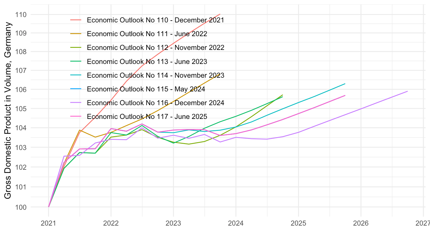
EO110_INTERNET |>
  mutate(vintage = "Perspectives économiques No 110 - Décembre 2021") |>
  bind_rows(EO111_INTERNET |>
              mutate(vintage = "Perspectives économiques No 111 - June 2022")) |>
  bind_rows(EO112_INTERNET |>
              mutate(vintage = "Perspectives économiques No 112 - November 2022")) |>
  bind_rows(EO113_INTERNET |>
              mutate(vintage = "Perspectives économiques No 113 - June 2023")) |>
  bind_rows(EO114_INTERNET |>
              mutate(vintage = "Perspectives économiques No 114 - November 2023")) |>
  filter(VARIABLE == "GDPV",
         LOCATION == "DEU",
         FREQUENCY == "Q") |>
  bind_rows(EO_115_extract |>
              mutate(vintage = "Perspectives économiques No 115 - May 2024")) |>
  bind_rows(EO_116_extract |>
              mutate(vintage = "Perspectives économiques No 116 - December 2024")) |>
  bind_rows(EO_117_extract |>
              mutate(vintage = "Perspectives économiques No 117 - June 2025")) |>
  quarter_to_date() |>
  filter(date >= as.Date("2021-01-01")) |>
  group_by(vintage) |>
  mutate(obsValue = 100*obsValue/obsValue[date == as.Date("2021-01-01")]) |>
  ggplot() + geom_line(aes(x = date, y = obsValue, color = vintage)) +
  xlab("") + ylab("Gross Domestic Product in Volume, Germany") + theme_minimal() +
  scale_x_date(breaks = seq(1920, 2100, 1) |> paste0("-01-01") |> as.Date(),
               labels = date_format("%Y")) +
  theme(legend.position = c(0.2, 0.6),
        legend.title = element_blank()) +
  scale_y_log10(breaks = seq(20, 200, 1))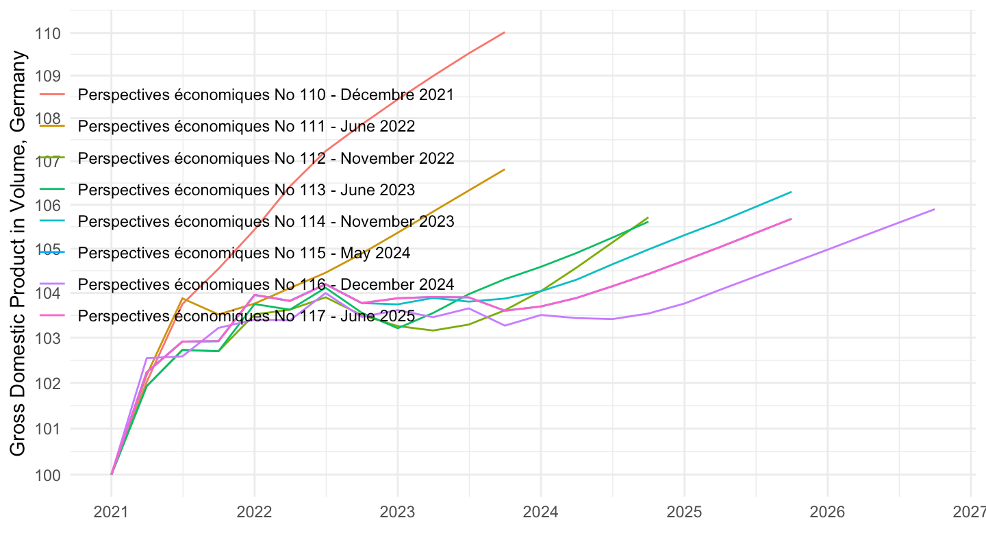
EO110_INTERNET |>
  mutate(vintage = "Perspectives économiques No 110 - Décembre 2021") |>
  filter(VARIABLE == "GDPV",
         LOCATION == "DEU",
         FREQUENCY == "Q") |>
  bind_rows(EO_117_extract |>
              mutate(vintage = "Perspectives économiques No 117 - Juin 2025")) |>
  quarter_to_date() |>
  filter(date >= as.Date("2021-01-01")) |>
  bind_rows(EO_117_extract |>
              mutate(vintage = "PIB réalisé") |>
              quarter_to_date() |>
              filter(date <= as.Date("2024-10-01"),
                     date >= as.Date("2021-01-01"))) |>
  group_by(vintage) |>
  mutate(obsValue = 100*obsValue/obsValue[date == as.Date("2021-01-01")]) |>
  ggplot() + geom_line(aes(x = date, y = obsValue, linetype = vintage)) +
  xlab("") + ylab("PIB en volume, Allemagne") + theme_minimal() +
  scale_x_date(breaks = seq(1920, 2100, 1) |> paste0("-01-01") |> as.Date(),
               labels = date_format("%Y")) +
  theme(legend.position = c(0.7, 0.2),
        legend.title = element_blank()) +
  scale_y_log10(breaks = seq(20, 200, 1))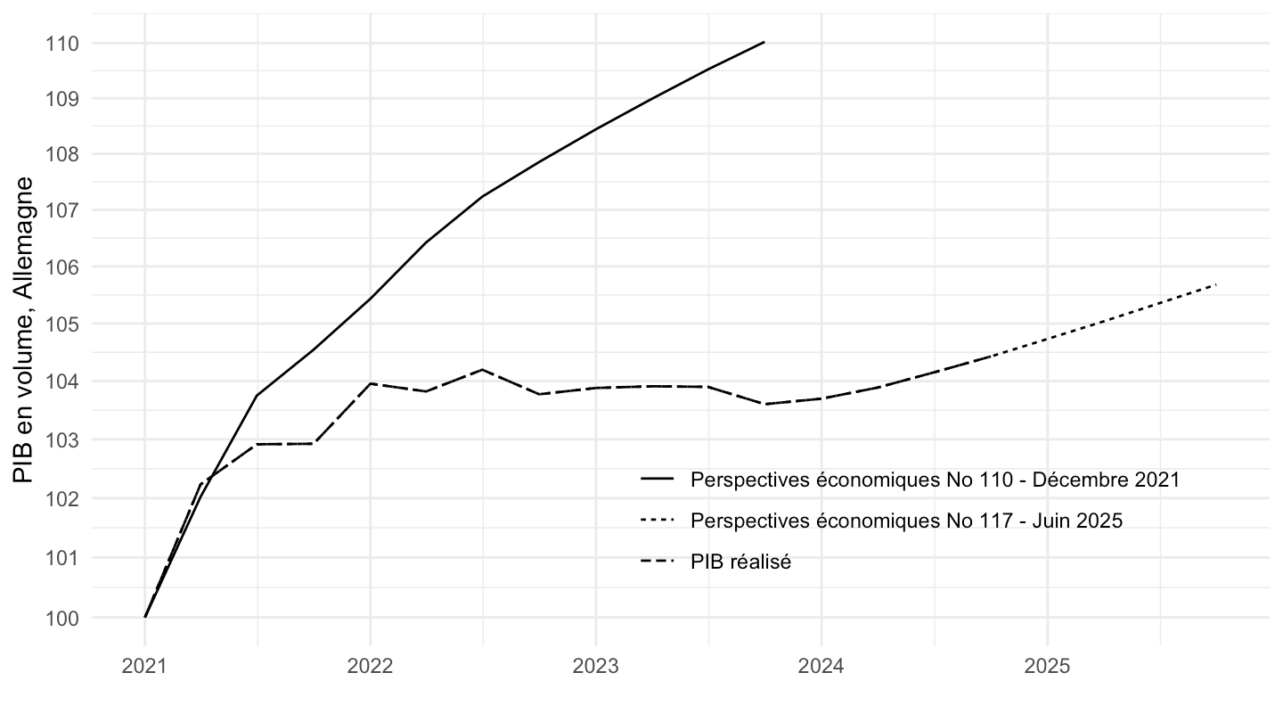
EO110_INTERNET |>
  mutate(vintage = "Economic Outlook No 110 - December 2021") |>
  bind_rows(EO111_INTERNET |>
              mutate(vintage = "Economic Outlook No 111 - June 2022")) |>
  bind_rows(EO112_INTERNET |>
              mutate(vintage = "Economic Outlook No 112 - November 2022")) |>
  bind_rows(EO113_INTERNET |>
              mutate(vintage = "Economic Outlook No 113 - June 2023")) |>
  bind_rows(EO114_INTERNET |>
              mutate(vintage = "Economic Outlook No 114 - November 2023")) |>
  filter(VARIABLE == "GDPV",
         LOCATION == "USA",
         FREQUENCY == "Q") |>
  quarter_to_date() |>
  filter(date >= as.Date("2021-01-01")) |>
  group_by(vintage) |>
  mutate(obsValue = 100*obsValue/obsValue[date == as.Date("2021-01-01")]) |>
  ggplot() + geom_line(aes(x = date, y = obsValue, color = vintage)) +
  xlab("") + ylab("Gross Domestic Product in Volume, United States") + theme_minimal() +
  scale_x_date(breaks = seq(1920, 2100, 1) |> paste0("-01-01") |> as.Date(),
               labels = date_format("%Y")) +
  theme(legend.position = c(0.7, 0.2),
        legend.title = element_blank()) +
  scale_y_log10(breaks = seq(20, 200, 1))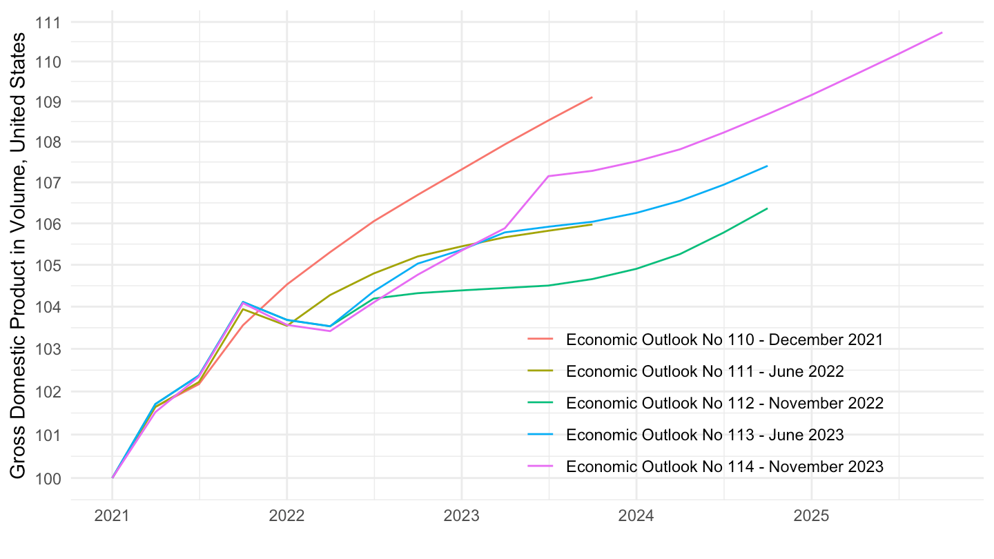
EO110_INTERNET |>
  mutate(vintage = "Economic Outlook No 110 - December 2021") |>
  bind_rows(EO111_INTERNET |>
              mutate(vintage = "Economic Outlook No 111 - June 2022")) |>
  bind_rows(EO112_INTERNET |>
              mutate(vintage = "Economic Outlook No 112 - November 2022")) |>
  bind_rows(EO113_INTERNET |>
              mutate(vintage = "Economic Outlook No 113 - June 2023")) |>
  bind_rows(EO114_INTERNET |>
              mutate(vintage = "Economic Outlook No 114 - November 2023")) |>
  filter(VARIABLE == "CPV",
         LOCATION == "DEU",
         FREQUENCY == "Q") |>
  quarter_to_date() |>
  filter(date >= as.Date("2021-01-01")) |>
  group_by(vintage) |>
  mutate(obsValue = 100*obsValue/obsValue[date == as.Date("2021-01-01")]) |>
  ggplot() + geom_line(aes(x = date, y = obsValue, color = vintage)) +
  xlab("") + ylab("Consumption in Volume, Germany") + theme_minimal() +
  scale_x_date(breaks = seq(1920, 2100, 1) |> paste0("-01-01") |> as.Date(),
               labels = date_format("%Y")) +
  theme(legend.position = c(0.7, 0.2),
        legend.title = element_blank()) +
  scale_y_log10(breaks = seq(20, 200, 1))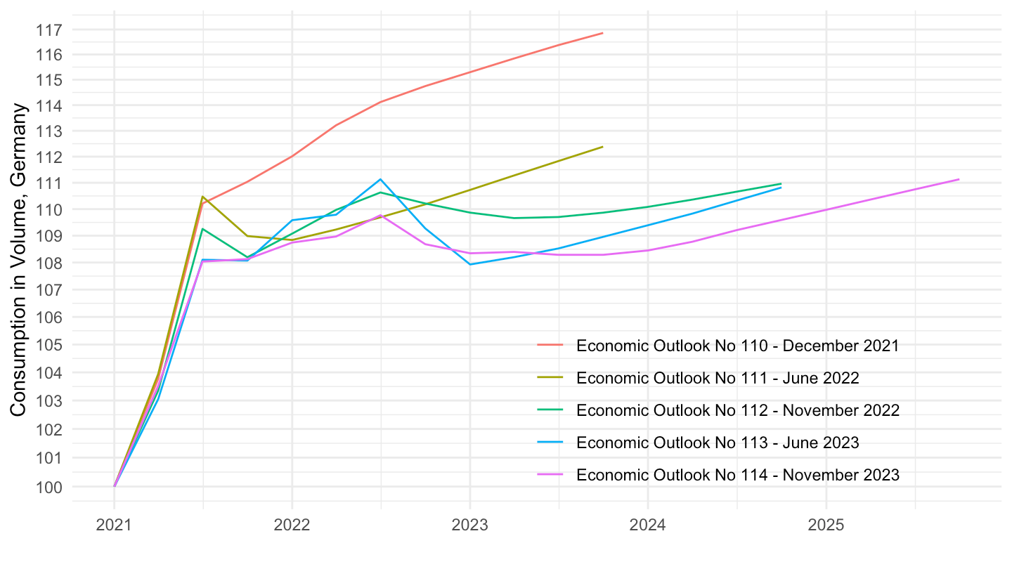
EO110_INTERNET |>
  mutate(vintage = "Economic Outlook No 110 - December 2021") |>
  bind_rows(EO111_INTERNET |>
              mutate(vintage = "Economic Outlook No 111 - June 2022")) |>
  bind_rows(EO112_INTERNET |>
              mutate(vintage = "Economic Outlook No 112 - November 2022")) |>
  bind_rows(EO113_INTERNET |>
              mutate(vintage = "Economic Outlook No 113 - June 2023")) |>
  bind_rows(EO114_INTERNET |>
              mutate(vintage = "Economic Outlook No 114 - November 2023")) |>
  filter(VARIABLE == "ITV",
         LOCATION == "DEU",
         FREQUENCY == "Q") |>
  quarter_to_date() |>
  filter(date >= as.Date("2021-01-01")) |>
  group_by(vintage) |>
  mutate(obsValue = 100*obsValue/obsValue[date == as.Date("2021-01-01")]) |>
  ggplot() + geom_line(aes(x = date, y = obsValue, color = vintage)) +
  xlab("") + ylab("Investment in Volume, Germany") + theme_minimal() +
  scale_x_date(breaks = seq(1920, 2100, 1) |> paste0("-01-01") |> as.Date(),
               labels = date_format("%Y")) +
  theme(legend.position = c(0.7, 0.2),
        legend.title = element_blank()) +
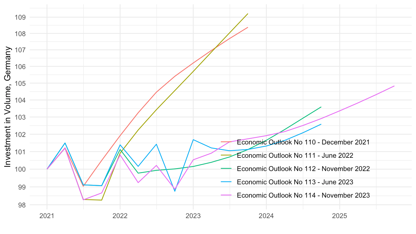
  scale_y_log10(breaks = seq(20, 200, 1))