Population and Labour Force - ALFS_POP_LABOUR

Data - OECD

Author

SUBJECT

Code

ALFS_POP_LABOUR %>%
  left_join(ALFS_POP_LABOUR_var$SUBJECT, by = "SUBJECT") %>%
  group_by(SUBJECT, Subject) %>%
  summarise(Nobs = n()) %>%
  arrange(-Nobs) %>%
  print_table_conditional()

SEX

Code

ALFS_POP_LABOUR %>%
  left_join(ALFS_POP_LABOUR_var$SEX, by = "SEX") %>%
  group_by(SEX, Sex) %>%
  summarise(Nobs = n()) %>%
  arrange(-Nobs) %>%
  print_table_conditional()

SEX	Sex	Nobs
TT	All persons	48889
MA	Males	39198
FE	Females	39020

LOCATION

Code

ALFS_POP_LABOUR %>%
  left_join(ALFS_POP_LABOUR_var$LOCATION, by = "LOCATION") %>%
  group_by(LOCATION, Location) %>%
  summarise(Nobs = n()) %>%
  arrange(-Nobs) %>%
  mutate(Flag = gsub(" ", "-", str_to_lower(gsub(" ", "-", Location))),
         Flag = paste0('<img src="../../icon/flag/vsmall/', Flag, '.png" alt="Flag">')) %>%
  select(Flag, everything()) %>%
  {if (is_html_output()) datatable(., filter = 'top', rownames = F, escape = F) else .}

Unemployment rate as % civilian labour force

Code

ALFS_POP_LABOUR %>%
  filter(SUBJECT == "YT99UNPT_ST", 
         SEX == "TT") %>%
  mutate(obsValue = obsValue %>% round(1) %>% paste("%")) %>%
  left_join(ALFS_POP_LABOUR_var$LOCATION, by = "LOCATION") %>%
  group_by(Location) %>%
  summarise(year_first = first(obsTime),
            value_first = first(obsValue),
            year_last = last(obsTime),
            value_last = last(obsValue)) %>%
  {if (is_html_output()) datatable(., filter = 'top', rownames = F) else .}

Employment / Population ratio

Code

ALFS_POP_LABOUR %>%
  # YT99CEL1_ST: Civilian employment
  # YP99TTL1_ST: Population
  filter(SUBJECT %in% c("YT99CEL1_ST", "YP99TTL1_ST"), 
         SEX == "TT") %>%
  select(LOCATION, obsTime, SUBJECT, obsValue, obsTime) %>%
  group_by(LOCATION, obsTime) %>%
  arrange(SUBJECT) %>%
  summarise(obsValue = obsValue[2]/ obsValue[1]) %>%
  na.omit %>%
  mutate(obsValue = (100*obsValue) %>% round(1) %>% paste("%")) %>%
  left_join(ALFS_POP_LABOUR_var$LOCATION, by = "LOCATION") %>%
  group_by(Location) %>%
  summarise(`Year 1` = first(obsTime),
            `Value 1` = first(obsValue),
            `Year 2` = last(obsTime),
            `Value 2` = last(obsValue)) %>%
  {if (is_html_output()) datatable(., filter = 'top', rownames = F) else .}

European Example

Code

ALFS_POP_LABOUR %>%
  filter(SUBJECT == "YT99CEP2_ST", 
         SEX == "TT",
         LOCATION %in% c("ITA", "DEU", "GRC", "ESP", "PRT", "FRA")) %>%
  year_to_date %>%
  filter(date >= as.Date("2000-01-01")) %>%
  left_join(ALFS_POP_LABOUR_var$LOCATION, by = "LOCATION") %>%
  group_by(LOCATION) %>%
  arrange(date) %>%
  mutate(obsValue = 100 * obsValue / obsValue[date == as.Date("2007-01-01")]) %>%
  ggplot(.) + geom_line(aes(x = date, y = obsValue, color = Location, linetype = Location)) + 
  scale_color_manual(values = viridis(7)[1:6]) +
  theme_minimal() + xlab("") + ylab("") +
  scale_x_date(breaks = seq(1960, 2020, 1) %>% paste0("-01-01") %>% as.Date,
               labels = date_format("%y")) +
  theme(legend.position = c(0.25, 0.9),
        legend.title = element_blank(),
        legend.direction = "horizontal") +
  scale_y_log10(breaks = seq(70, 200, 5))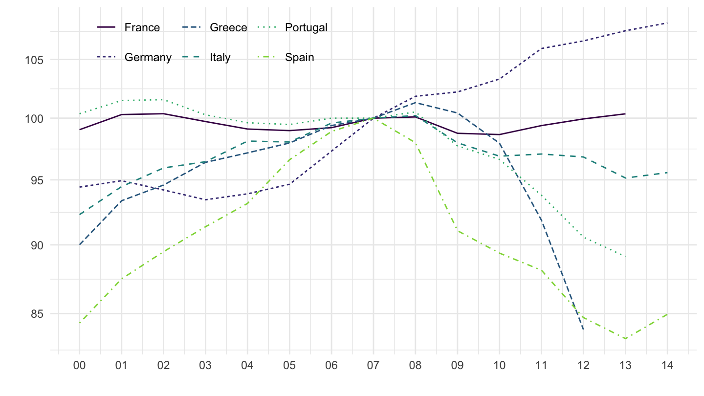

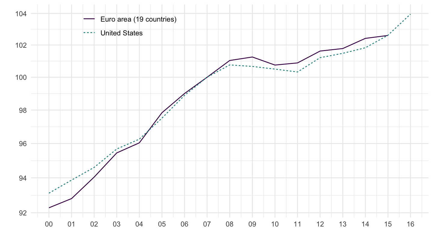
Civilian labour force, Index

Code

ALFS_POP_LABOUR %>%
  filter(SUBJECT == "YG9907L1_IXOB", 
         SEX == "TT",
         LOCATION %in% c("EA19", "USA")) %>%
  year_to_date %>%
  filter(date >= as.Date("2000-01-01")) %>%
  left_join(ALFS_POP_LABOUR_var$LOCATION, by = "LOCATION") %>%
  group_by(LOCATION) %>%
  arrange(date) %>%
  mutate(obsValue = 100 * obsValue / obsValue[date == as.Date("2007-01-01")]) %>%
  ggplot(.) + geom_line(aes(x = date, y = obsValue, color = Location, linetype = Location)) + 
  scale_color_manual(values = viridis(3)[1:2]) +
  theme_minimal() + xlab("") + ylab("") +
  scale_x_date(breaks = seq(1960, 2020, 1) %>% paste0("-01-01") %>% as.Date,
               labels = date_format("%y")) +
  theme(legend.position = c(0.25, 0.9),
        legend.title = element_blank()) +
  scale_y_log10(breaks = seq(70, 200, 2))