Microprocessor Trend Data

Data - Log

Author

Info

Microprocessor Trend Data html

LAST_COMPILE

LAST_COMPILE
2024-06-20

variable

Code

`microprocessor-trend-data` %>%
  group_by(variable) %>%
  summarise(Nobs = n()) %>%
  print_table_conditional()

variable	Nobs
cores	91
frequency	102
specint	76
transistors	100
watts	102

Transistors

Linear

Code

plot_linear <- `microprocessor-trend-data` %>%
  filter(variable == "transistors") %>%
  transmute(V1 = as.numeric(V1),
            V2 = V2) %>%
  filter(!is.na(V1), !is.na(V2)) %>%
  ggplot + geom_line(aes(x = V1, y = V2)) +
  scale_y_continuous(breaks = 10^7*seq(0, 10, 1)) +
  theme_minimal()  +
  ylab("# of transistors per microprocessor") + xlab("")

plot_linear

Log

Code

plot_log <- plot_linear +
  scale_y_log10(breaks = 10^(seq(1, 10, 1)))

plot_log

Both

Code

ggarrange(plot_linear + ggtitle("Moore's Law\nLinear Scale"),
          plot_log + ggtitle("\nLog Scale") + ylab(""))

Watts

Both

Code

plot1 <- `microprocessor-trend-data` %>%
  filter(variable == "watts") %>%
  transmute(V1 = as.numeric(V1),
            V2 = V2) %>%
  filter(!is.na(V1), !is.na(V2)) %>%
  ggplot + geom_line(aes(x = V1, y = V2)) +
  scale_y_continuous(breaks = seq(0, 1000, 50)) +
  theme_minimal() + ggtitle("Linear Scale") +
  ylab("Watts") + xlab("")


plot2 <- plot1 +
  scale_y_log10(breaks = c(1, 2, 5, 8, 10, 20, 50, 80, 100, 200, 500)) +
  ggtitle("Log Scale")

ggarrange(plot1, plot2)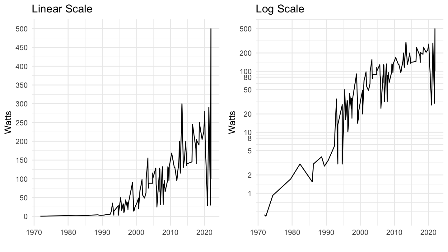

Linear

Code

plot1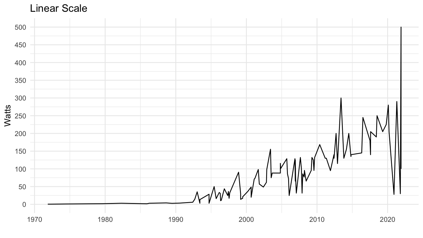

Log

Code

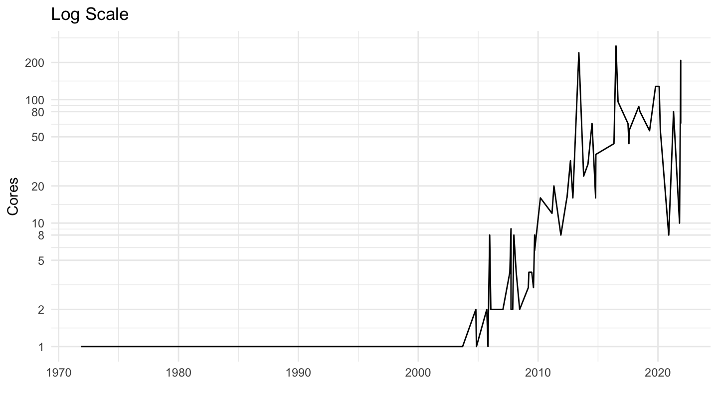
plot2

Cores

Both

Code

plot1 <- `microprocessor-trend-data` %>%
  filter(variable == "cores") %>%
  transmute(V1 = as.numeric(V1),
            V2 = V2) %>%
  filter(!is.na(V1), !is.na(V2)) %>%
  ggplot + geom_line(aes(x = V1, y = V2)) +
  scale_y_continuous(breaks = seq(0, 1000, 50)) +
  theme_minimal() + ggtitle("Linear Scale") +
  ylab("Cores") + xlab("")


plot2 <- plot1 +
  scale_y_log10(breaks = c(1, 2, 5, 8, 10, 20, 50, 80, 100, 200, 500)) +
  ggtitle("Log Scale")

ggarrange(plot1, plot2)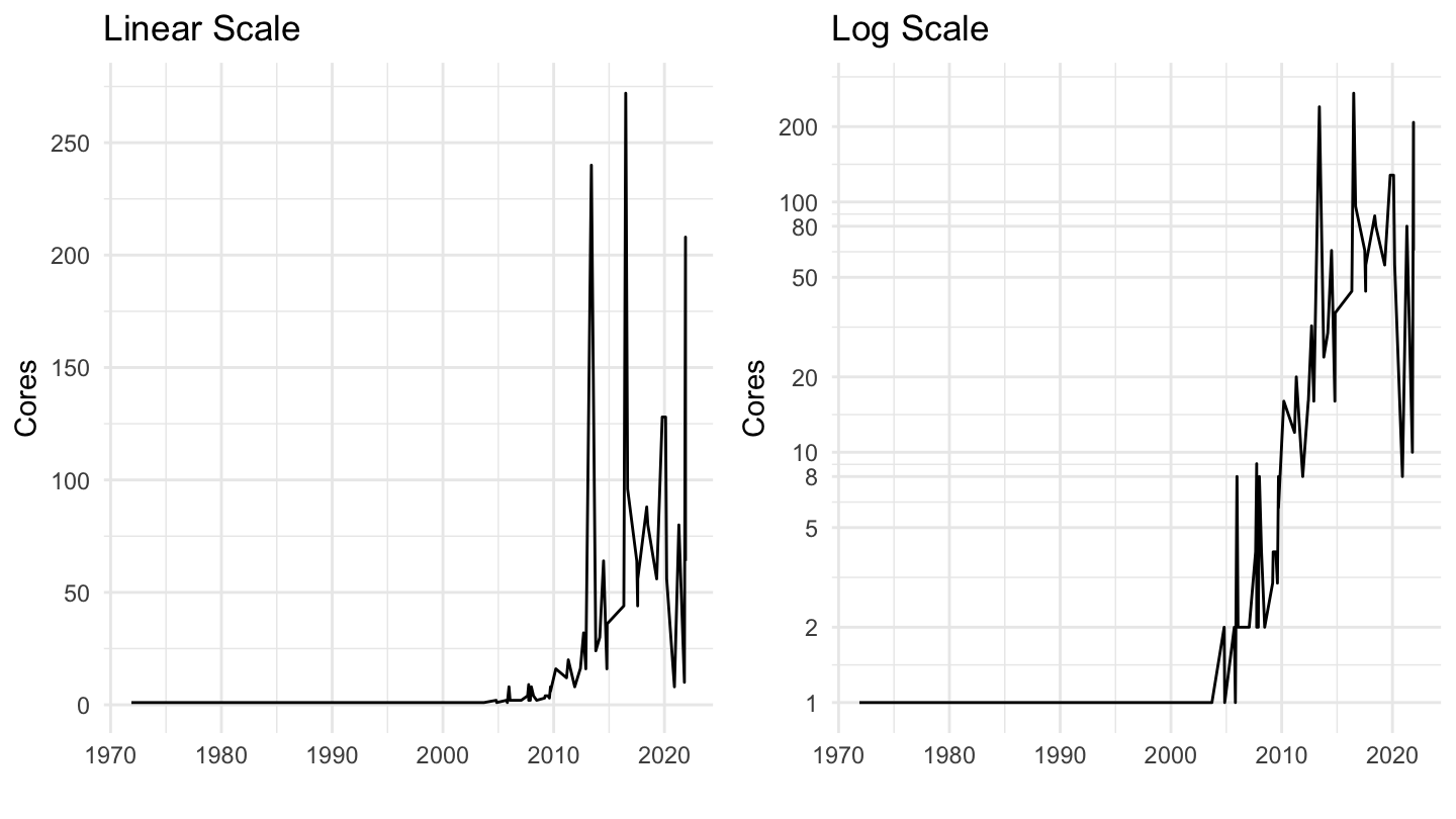

Linear

Code

plot1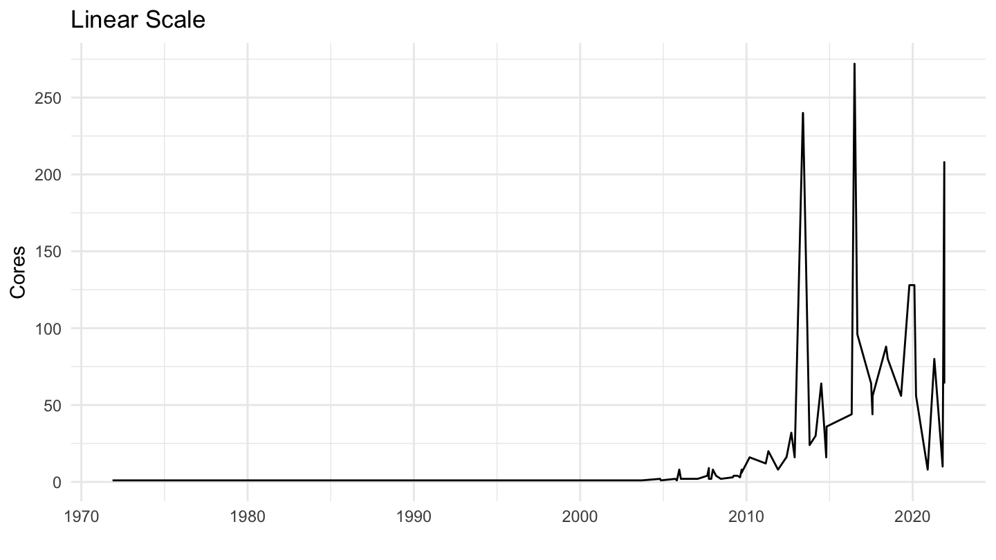

Log

Code

plot2