John Fernald TFP - john-fernald-tfp

Data

Author

variable

Annual

Code

annual_tfp %>%
  left_join(variable, by = "variable") %>%
  group_by(variable, Variable) %>%
  summarise(Nobs = n()) %>%
  print_table_conditional()

variable	Variable	Nobs
alpha	Capital's share of income	73
dLP	Business- sector labor productivity	73
dLQ	Labor composition/quality actually used	73
dLQ_Aaronson_Sullivan	NA	73
dLQ_BLS_interpolated	Labor composition/quality from BLS	73
dY	Output	73
dY_inc	Business output, measured from income side	73
dY_prod	Business output, expenditure (product) side	73
dhours	Hours, bus sector	73
dk	Capital input	73
dtfp	Business sector TFP	73
dtfp_C	TFP in non-equipment business output ("consumption")	73
dtfp_C_util	Utilization-adjusted TFP in producing non-equipment output	73
dtfp_I	TFP in equip and consumer durables	73
dtfp_I_util	Utilization-adjusted TFP in producing equipment and consumer durables	73
dtfp_util	Utilization-adjusted TFP	73
du_consumption	Utilization in producing non-investment business output ("consumption")	73
du_invest	Utilization in producing investment	73
dutil	Utilization of capital and labor	73
invShare	Equipment and consumer durables share of output	73
relativePrice	Relative price of "consumption" to price of "equipment"	73

Quarterly

Code

quarterly_tfp %>%
  left_join(variable, by = "variable") %>%
  group_by(variable, Variable) %>%
  summarise(Nobs = n()) %>%
  print_table_conditional()

variable	Variable	Nobs
alpha	Capital's share of income	297
dLP	Business- sector labor productivity	296
dLQ	Labor composition/quality actually used	296
dLQ_Aaronson_Sullivan	NA	168
dLQ_BLS_interpolated	Labor composition/quality from BLS	296
dY	Output	296
dY_inc	Business output, measured from income side	296
dY_prod	Business output, expenditure (product) side	296
dhours	Hours, bus sector	296
dk	Capital input	296
dtfp	Business sector TFP	296
dtfp_C	TFP in non-equipment business output ("consumption")	296
dtfp_C_util	Utilization-adjusted TFP in producing non-equipment output	296
dtfp_I	TFP in equip and consumer durables	296
dtfp_I_util	Utilization-adjusted TFP in producing equipment and consumer durables	296
dtfp_util	Utilization-adjusted TFP	296
du_consumption	Utilization in producing non-investment business output ("consumption")	296
du_invest	Utilization in producing investment	296
dutil	Utilization of capital and labor	296
invShare	Equipment and consumer durables share of output	297
month	NA	297
relativePrice	Relative price of "consumption" to price of "equipment"	296

Quarterly

Code

quarterly_tfp %>%
  filter(variable %in% c("dtfp", "dtfp_util")) %>%
  left_join(variable, by = "variable") %>%
  ggplot + theme_minimal() + xlab("") + ylab("") +
  geom_line(aes(x = date, y = value, color = Variable)) +
  scale_x_date(breaks = seq(1920, 2025, 5) %>% paste0("-01-01") %>% as.Date,
               labels = date_format("%y")) +
  scale_y_continuous(breaks = c(seq(-200, 100, 2))) +
  theme(legend.position = c(0.25, 0.9),
        legend.title = element_blank()) + 
  scale_color_manual(values = viridis(3)[1:2])

Annual

Code

annual_tfp %>%
  filter(variable %in% c("dtfp", "dtfp_util")) %>%
  left_join(variable, by = "variable") %>%
  ggplot + theme_minimal() + xlab("") + ylab("TFP growth (%)") +
  geom_line(aes(x = date, y = value /100, color = Variable)) +
  scale_x_date(breaks = seq(1920, 2025, 5) %>% paste0("-01-01") %>% as.Date,
               labels = date_format("%y")) +
  scale_y_continuous(breaks = 0.01*c(seq(-200, 100, 1)),
                     labels = scales::percent_format(accuracy = 1)) +
  geom_rect(data = nber_recessions %>%
              filter(Peak > as.Date("1945-01-01")), 
            aes(xmin = Peak, xmax = Trough, ymin = -Inf, ymax = +Inf), 
            fill = 'grey', alpha = 0.5) +
  theme(legend.position = c(0.8, 0.9),
        legend.title = element_blank()) + 
  scale_color_manual(values = viridis(3)[1:2])

5-year TFP Growth

Line

Code

annual_tfp %>%
  filter(variable %in% c("dtfp", "dtfp_util")) %>%
  left_join(variable, by = "variable") %>%
  group_by(variable) %>%
  mutate(value = value/100,
         value_5Y = ((1+value)*(1+lag(value))*(1+lag(value, 2))*(1+lag(value, 3))*(1+lag(value, 4)))^(1/5)-1) %>%
  na.omit %>%
  ggplot + theme_minimal() + xlab("") + ylab("5-year previous TFP growth (%)") +
  geom_line(aes(x = date, y = value_5Y, color = Variable)) +
  scale_x_date(breaks = seq(1920, 2025, 5) %>% paste0("-01-01") %>% as.Date,
               labels = date_format("%y")) +
  scale_y_continuous(breaks = 0.01*c(seq(-200, 100, 0.5)),
                     labels = scales::percent_format(accuracy = .1)) +
  geom_rect(data = nber_recessions %>%
              filter(Peak > as.Date("1950-01-01")), 
            aes(xmin = Peak, xmax = Trough, ymin = -Inf, ymax = +Inf), 
            fill = 'grey', alpha = 0.5) +
  theme(legend.position = c(0.8, 0.9),
        legend.title = element_blank()) + 
  scale_color_manual(values = viridis(3)[1:2])

Scatter

Code

annual_tfp %>%
  filter(variable %in% c("dtfp", "dtfp_util")) %>%
  left_join(variable, by = "variable") %>%
  group_by(variable) %>%
  mutate(value = value/100,
         value_5Y = ((1+value)*(1+lag(value))*(1+lag(value, 2))*(1+lag(value, 3))*(1+lag(value, 4)))^(1/5)-1) %>%
  na.omit %>%
  ggplot + theme_minimal() + xlab("") + ylab("5-year previous TFP growth (%)") +
  geom_point(aes(x = date, y = value_5Y, color = Variable)) +
  scale_x_date(breaks = seq(1920, 2025, 5) %>% paste0("-01-01") %>% as.Date,
               labels = date_format("%y")) +
  scale_y_continuous(breaks = 0.01*c(seq(-200, 100, 0.5)),
                     labels = scales::percent_format(accuracy = .1)) +
  geom_rect(data = nber_recessions %>%
              filter(Peak > as.Date("1950-01-01")), 
            aes(xmin = Peak, xmax = Trough, ymin = -Inf, ymax = +Inf), 
            fill = 'grey', alpha = 0.5) +
  theme(legend.position = c(0.8, 0.9),
        legend.title = element_blank()) + 
  scale_color_manual(values = viridis(3)[1:2])

10-year TFP Growth

Code

annual_tfp %>%
  filter(variable %in% c("dtfp", "dtfp_util")) %>%
  left_join(variable, by = "variable") %>%
  group_by(variable) %>%
  mutate(value = value/100,
         value_5Y = ((1+value)*(1+lag(value))*(1+lag(value, 2))*(1+lag(value, 3))*(1+lag(value, 4))*(1+lag(value, 5))*(1+lag(value, 6))*(1+lag(value, 7))*(1+lag(value, 8))*(1+lag(value, 9)))^(1/10)-1) %>%
  na.omit %>%
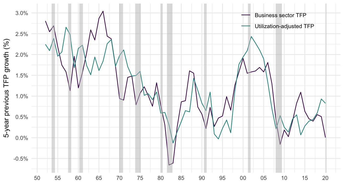
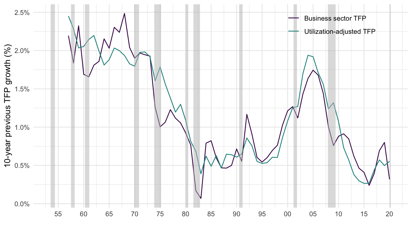
  ggplot + theme_minimal() + xlab("") + ylab("10-year previous TFP growth (%)") +
  geom_line(aes(x = date, y = value_5Y, color = Variable)) +
  scale_x_date(breaks = seq(1920, 2025, 5) %>% paste0("-01-01") %>% as.Date,
               labels = date_format("%y")) +
  scale_y_continuous(breaks = 0.01*c(seq(-200, 100, 0.5)),
                     labels = scales::percent_format(accuracy = .1)) +
  geom_rect(data = nber_recessions %>%
              filter(Peak > as.Date("1950-01-01")), 
            aes(xmin = Peak, xmax = Trough, ymin = -Inf, ymax = +Inf), 
            fill = 'grey', alpha = 0.5) +
  theme(legend.position = c(0.8, 0.9),
        legend.title = element_blank()) + 
  scale_color_manual(values = viridis(3)[1:2])