Stocks

Data - Investing

Nobs

stocks %>%
  filter(country == "france") %>%
  select(name, symbol) %>%
  {if (is_html_output()) datatable(., filter = 'top', rownames = F) else .}

KOHL: Kehrig (Gucci, YSL), L’Oréal, Hermes, LVMH

Stock Prices

stocks_FRA %>%
  filter(symbol %in% c("ADP", "RENA", "EDF")) %>%
  left_join(stocks_FRA_var, by = "symbol") %>%
  ggplot + geom_line(aes(x = Date, y = Close, color = full_name)) + 
  theme_minimal() + xlab("") + ylab("Stock Price (Close)") +
  scale_x_date(breaks = seq(1960, 2020, 2) %>% paste0("-01-01") %>% as.Date,
               labels = date_format("%y")) +
  scale_y_log10(breaks = c(1, 2, 3, 5, 10, 25, 50, 100, 200, 500),
                     labels = dollar_format(prefix = "", suffix = "€", accuracy = 1)) +
  scale_color_manual(values = viridis(5)[1:4]) +
  theme(legend.position = c(0.2, 0.80),
        legend.title = element_blank())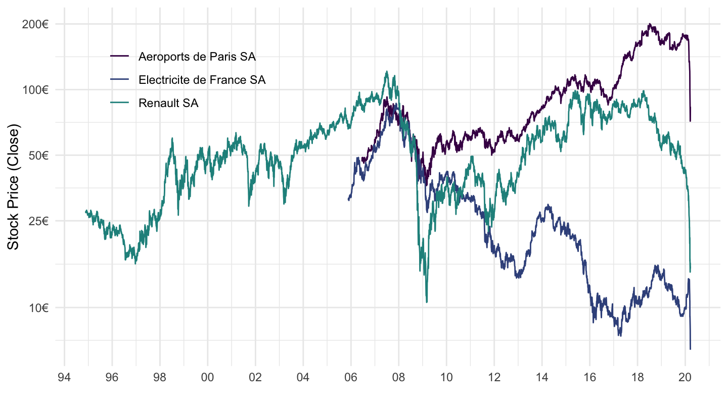

CAC40 in France

indices_FRA %>%
  filter(symbol %in% c("FCHI")) %>%
  select(Date, CAC40 = Close) %>%
  ggplot + geom_line(aes(x = Date, y = CAC40)) + 
  theme_minimal() + xlab("") + ylab("") +
  scale_x_date(breaks = seq(1960, 2020, 2) %>% paste0("-01-01") %>% as.Date,
               labels = date_format("%y")) +
  scale_y_log10(breaks = seq(0, 20000, 1000)) +
  scale_color_manual(values = viridis(5)[1:4]) +
  theme(legend.position = c(0.2, 0.85),
        legend.title = element_blank())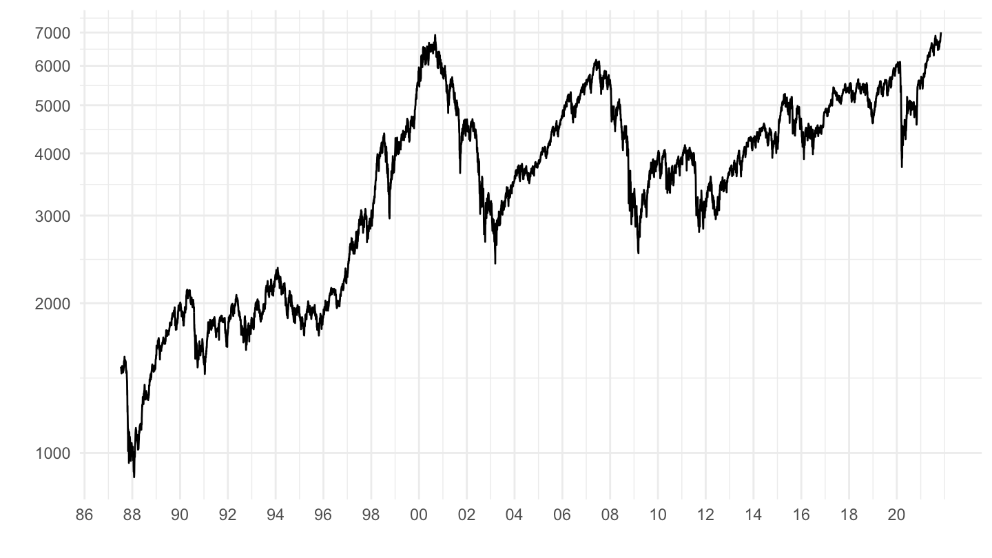

Essai CAPM

data <- stocks_FRA %>%
  select(symbol, Date, Close) %>%
  left_join(indices_FRA %>%
              filter(symbol %in% c("FCHI")) %>%
              select(Date, CAC40 = Close), 
            by = "Date") %>%
  group_by(symbol) %>%
  complete(Date = seq.Date(min(Date), max(Date), by = "day")) %>%
  fill(Close, CAC40) %>%
  filter(!is.na(CAC40),
         day(Date) == 1) %>%
  mutate_at(vars(Close, CAC40), funs(log(.) - lag(log(.), 1))) %>%
  group_by(symbol) %>%
  na.omit %>%
  summarise(covariance = cov(Close, CAC40) / cov(CAC40, CAC40),
            mean = exp(12*mean(Close))-1,
            first = first(Date),
            last = last(Date))

Betas

data %>%
  filter(first == as.Date("1987-09-01")) %>%
  ggplot(.) + theme_minimal() + 
  geom_point(aes(x = covariance, y = mean)) +
  geom_text_repel(aes(x = covariance, y = mean, label = symbol)) +
  xlab("Beta") + ylab("Return") +
  scale_x_continuous(breaks = seq(0, 4, 0.1)) +
  scale_y_continuous(breaks = 0.01*seq(-20, 20, 1),
                     labels = scales::percent_format(accuracy = 1)) +
  stat_smooth(aes(x = covariance, y = mean), linetype = 2, method = "lm", color = viridis(3)[2])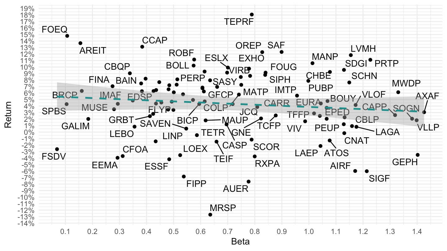

data %>%
  filter(first == as.Date("1987-09-01")) %>%
  ggplot(.) + theme_minimal() + 
  geom_point(aes(x = covariance, y = mean)) +
  geom_text_repel(aes(x = covariance, y = mean, label = symbol)) +
  xlab("Beta") + ylab("Return") +
  scale_x_continuous(breaks = seq(0, 4, 0.1)) +
  scale_y_continuous(breaks = 0.01*seq(-20, 20, 1),
                     labels = scales::percent_format(accuracy = 1)) +
  stat_smooth(aes(x = covariance, y = mean), linetype = 2, method = "lm", color = viridis(3)[2])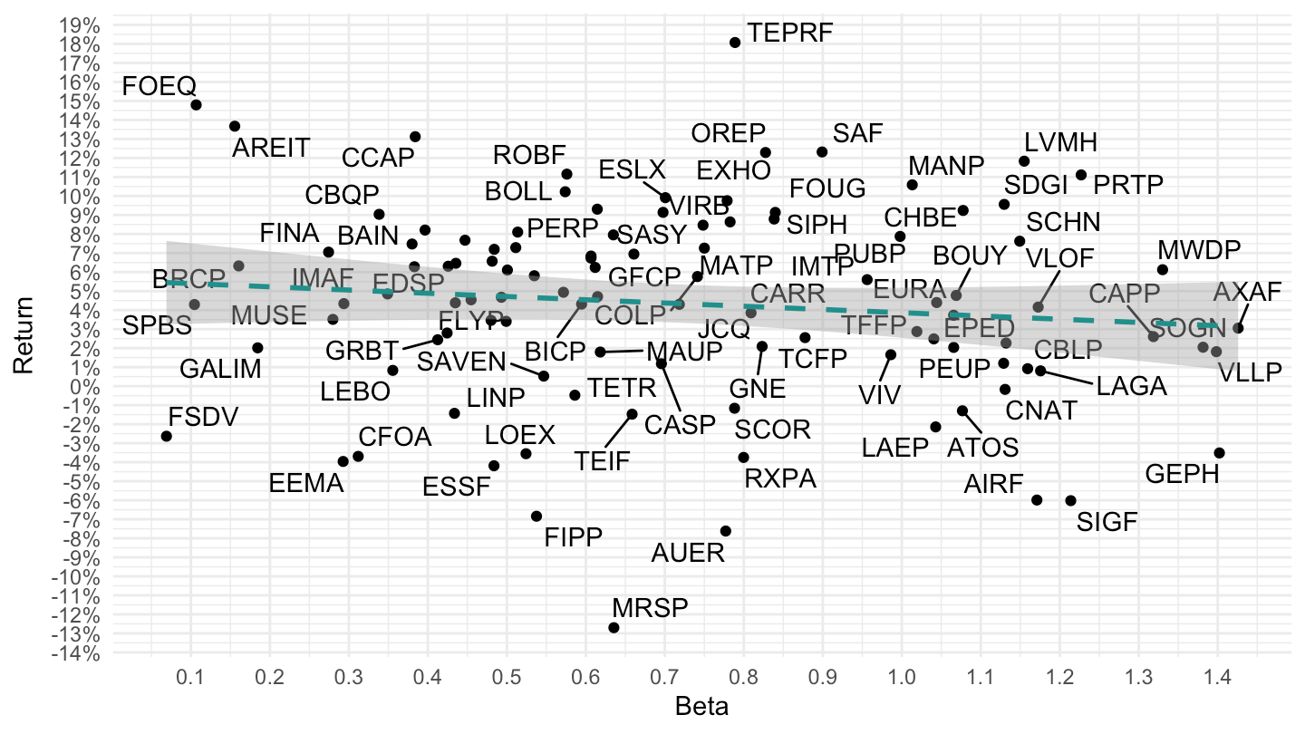

data %>%
  left_join(stocks %>%
              select(symbol, name), by = "symbol") %>%
  filter(first == as.Date("1987-09-01")) %>%
  ggplot(.) + theme_minimal() + 
  geom_point(aes(x = covariance, y = mean)) +
  geom_text_repel(aes(x = covariance, y = mean, label = name)) +
  xlab("Beta") + ylab("Return") +
  scale_x_continuous(breaks = seq(0, 4, 0.1)) +
  scale_y_continuous(breaks = 0.01*seq(-20, 20, 1),
                     labels = scales::percent_format(accuracy = 1)) +
  stat_smooth(aes(x = covariance, y = mean), linetype = 2, method = "lm", color = viridis(3)[2])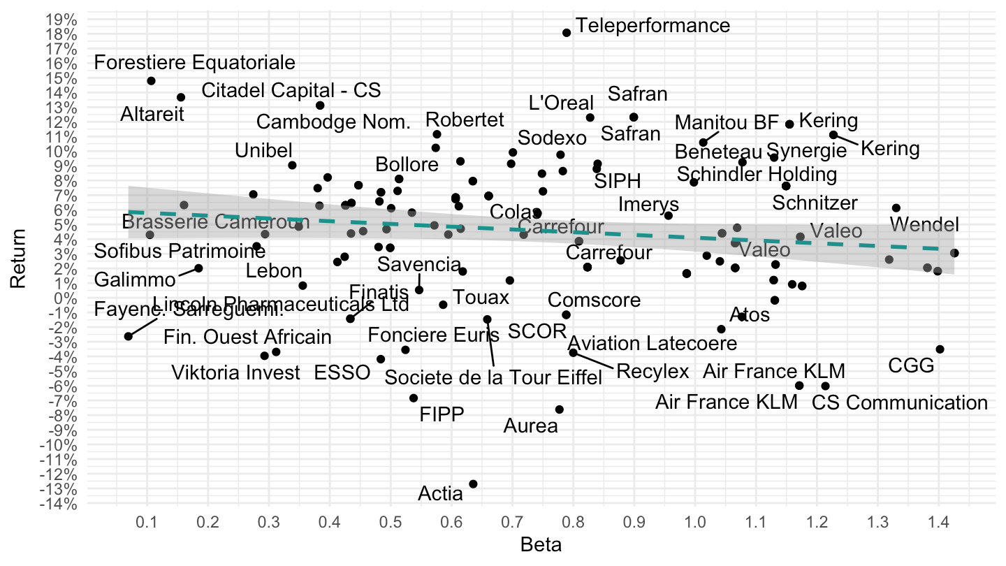

data %>%
  filter(first == as.Date("1987-09-01")) %>%
  lm(mean ~ covariance, data = .) %>%
  summary

# 
# Call:
# lm(formula = mean ~ covariance, data = .)
# 
# Residuals:
#       Min        1Q    Median        3Q       Max 
# -0.171844 -0.024386 -0.000212  0.033190  0.138504 
# 
# Coefficients:
#             Estimate Std. Error t value Pr(>|t|)    
# (Intercept)  0.05566    0.01202   4.631 1.06e-05 ***
# covariance  -0.01704    0.01518  -1.123    0.264    
# ---
# Signif. codes:  0 '***' 0.001 '**' 0.01 '*' 0.05 '.' 0.1 ' ' 1
# 
# Residual standard error: 0.05197 on 103 degrees of freedom
# Multiple R-squared:  0.01209, Adjusted R-squared:  0.002501 
# F-statistic: 1.261 on 1 and 103 DF,  p-value: 0.2641

data %>%
  lm(mean ~ covariance, data = .) %>%
  summary

# 
# Call:
# lm(formula = mean ~ covariance, data = .)
# 
# Residuals:
#      Min       1Q   Median       3Q      Max 
# -0.79503 -0.08422  0.04277  0.11051  1.33026 
# 
# Coefficients:
#              Estimate Std. Error t value Pr(>|t|)    
# (Intercept) -0.042048   0.008444  -4.980 7.91e-07 ***
# covariance  -0.001514   0.006289  -0.241     0.81    
# ---
# Signif. codes:  0 '***' 0.001 '**' 0.01 '*' 0.05 '.' 0.1 ' ' 1
# 
# Residual standard error: 0.2042 on 746 degrees of freedom
#   (1 observation effacée parce que manquante)
# Multiple R-squared:  7.765e-05,   Adjusted R-squared:  -0.001263 
# F-statistic: 0.05793 on 1 and 746 DF,  p-value: 0.8099