Code
tibble(LAST_DOWNLOAD = as.Date(file.info("~/iCloud/website/data/investing/indices.RData")$mtime)) %>%
print_table_conditional()| LAST_DOWNLOAD |
|---|
| 2022-06-29 |
Data - Investing
tibble(LAST_DOWNLOAD = as.Date(file.info("~/iCloud/website/data/investing/indices.RData")$mtime)) %>%
print_table_conditional()| LAST_DOWNLOAD |
|---|
| 2022-06-29 |
| LAST_COMPILE |
|---|
| 2025-03-12 |
| Date | Nobs |
|---|---|
| 2022-06-29 | 1 |
Source: investing.com, March 12, 2025. [html]
ig_b("asset-pricing", "2021-11-06-the-economist")
indices_var %>%
  select(country, symbol, full_name) %>%
print_table_conditional()indices_var %>%
select(country, symbol, full_name, currency) %>%
filter(grepl("Total Return", full_name)) %>%
print_table_conditional()indices %>%
group_by(symbol) %>%
summarise(Nobs = n()) %>%
left_join(indices_var %>%
select(country, symbol, full_name, currency), by = "symbol") %>%
arrange(country) %>%
print_table_conditional()| symbol | Nobs | country | full_name | currency |
|---|---|---|---|---|
| BVSP | 5128 | brazil | Bovespa | BRL |
| FCHI | 8872 | france | CAC 40 | EUR |
| FRCS | 5998 | france | CAC Consumer Service | EUR |
| PX1GR | 8750 | france | CAC 40 Gross Total Return | EUR |
| PX1NR | 8750 | france | CAC 40 Net Total Return | EUR |
| PX4GR | 3390 | france | SBF 120 Gross Total Retrun | EUR |
| PX4NR | 3390 | france | SBF 120 Net Total Return | EUR |
| BKJPT | 4959 | japan | BNY Mellon Japan ADR Total Return | USD |
| N225TR | 2095 | japan | Nikkei 225 Total Return | JPY |
| BKEST | 4960 | spain | BNY Mellon Spain ADR Total Return | USD |
| IBEXTR | 2564 | spain | IBEX Total Return | EUR |
| BKGBT | 4962 | united kingdom | BNY Mellon United Kingdom ADR Total Return | USD |
| TRIUKX | 2240 | united kingdom | FTSE 100 Total Return | GBP |
| DJDVY | 1935 | united states | Dow Jones U.S. Select Dividend Total Return | USD |
| DJI | 10721 | united states | Dow Jones Industrial Average | USD |
| IXIC | 10662 | united states | NASDAQ Composite | USD |
| SPX | 10721 | united states | S&P 500 | USD |
| SPXGTR | 1602 | united states | S&P 500 Growth Total Return | USD |
| SPXTR | 5256 | united states | S&P 500 TR | USD |
| XCMP | 1932 | united states | NASDAQ Composite Total Return | USD |
| BKADR | 5066 | world | BNY Mellon ADR | USD |
| EE050L | 1573 | world | STOXX Eastern Europe 300 Oil & Gas USD Price | USD |
| EE950L | 1827 | world | STOXX Eastern Europe 300 Technology USD Price | USD |
| FTFQE | 1546 | world | FTSE Emerging Markets China A Inclusion | USD |
| MIWO00000PUS | 2434 | world | MSCI World | USD |
| MSCIEF | 2550 | world | MSCI Emerging Markets | USD |
indices %>%
  left_join(indices_var, by = "symbol") %>%
  group_by(symbol, full_name) %>%
  summarise(Nobs = n()) %>%
print_table_conditional()| symbol | full_name | Nobs |
|---|---|---|
| BKADR | BNY Mellon ADR | 5066 |
| BKEST | BNY Mellon Spain ADR Total Return | 4960 |
| BKGBT | BNY Mellon United Kingdom ADR Total Return | 4962 |
| BKJPT | BNY Mellon Japan ADR Total Return | 4959 |
| BVSP | Bovespa | 5128 |
| DJDVY | Dow Jones U.S. Select Dividend Total Return | 1935 |
| DJI | Dow Jones Industrial Average | 10721 |
| EE050L | STOXX Eastern Europe 300 Oil & Gas USD Price | 1573 |
| EE950L | STOXX Eastern Europe 300 Technology USD Price | 1827 |
| FCHI | CAC 40 | 8872 |
| FRCS | CAC Consumer Service | 5998 |
| FTFQE | FTSE Emerging Markets China A Inclusion | 1546 |
| IBEXTR | IBEX Total Return | 2564 |
| IXIC | NASDAQ Composite | 10662 |
| MIWO00000PUS | MSCI World | 2434 |
| MSCIEF | MSCI Emerging Markets | 2550 |
| N225TR | Nikkei 225 Total Return | 2095 |
| PX1GR | CAC 40 Gross Total Return | 8750 |
| PX1NR | CAC 40 Net Total Return | 8750 |
| PX4GR | SBF 120 Gross Total Retrun | 3390 |
| PX4NR | SBF 120 Net Total Return | 3390 |
| SPX | S&P 500 | 10721 |
| SPXGTR | S&P 500 Growth Total Return | 1602 |
| SPXTR | S&P 500 TR | 5256 |
| TRIUKX | FTSE 100 Total Return | 2240 |
| XCMP | NASDAQ Composite Total Return | 1932 |
indices %>%
  filter(symbol %in% c("FCHI", "PX1GR", "SPXTR", "SPX")) %>%
  left_join(indices_var, by = "symbol") %>%
  group_by(symbol) %>%
  mutate(Close = Close / Close[1]) %>%
  ggplot + geom_line(aes(x = Date, y = Close, color = paste(symbol, "-", name))) +
  theme_minimal() + xlab("") + ylab("") +
  scale_x_date(breaks = seq(1960, 2022, 2) %>% paste0("-01-01") %>% as.Date,
               labels = date_format("%y")) +
  scale_y_log10(breaks = seq(0, 20, 1)) +
  scale_color_manual(values = viridis(5)[1:4]) +
  theme(legend.position = c(0.2, 0.85),
        legend.title = element_blank())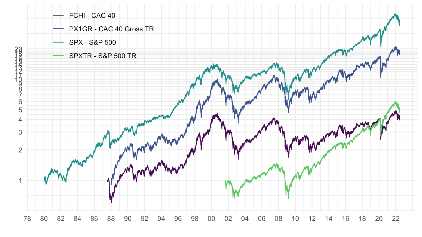
indices %>%
  filter(symbol %in% c("FCHI", "PX1GR", "SPXTR", "SPX")) %>%
  left_join(indices_var, by = "symbol") %>%
  filter(Date >= as.Date("2000-01-01")) %>%
  group_by(symbol) %>%
  mutate(Close = Close / Close[1]) %>%
  ggplot + geom_line(aes(x = Date, y = Close, color = paste(symbol, "-", name))) +
  theme_minimal() + xlab("") + ylab("") +
  scale_x_date(breaks = seq(1960, 2022, 5) %>% paste0("-01-01") %>% as.Date,
               labels = date_format("%Y")) +
  scale_y_log10(breaks = seq(0, 20, 1)) +
  scale_color_manual(values = viridis(5)[1:4]) +
  theme(legend.position = c(0.2, 0.85),
        legend.title = element_blank())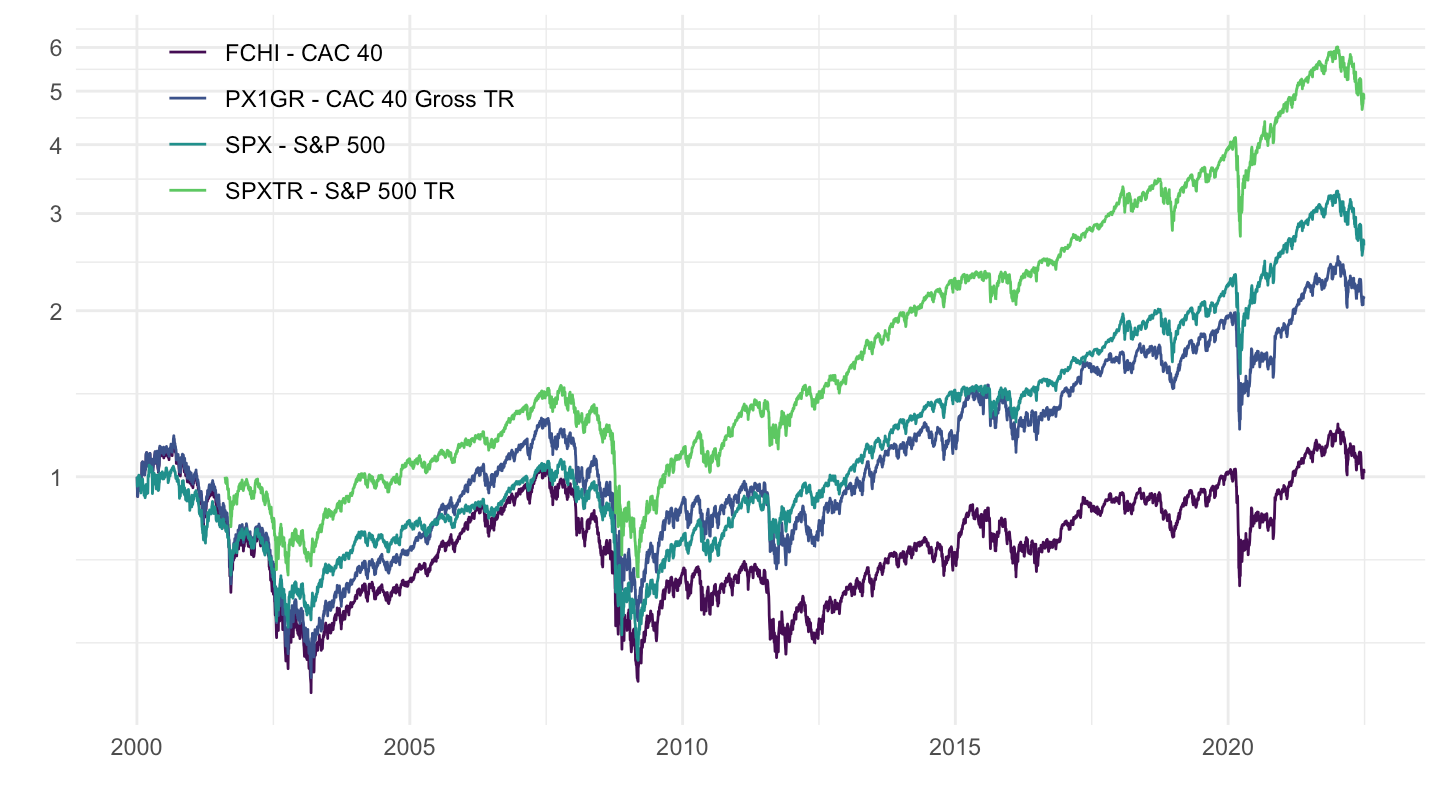
indices %>%
  filter(symbol %in% c("FCHI", "PX1GR", "SPXTR", "SPX")) %>%
  left_join(indices_var, by = "symbol") %>%
  filter(Date >= as.Date("2010-01-01")) %>%
  group_by(symbol) %>%
  mutate(Close = Close / Close[1]) %>%
  ggplot + geom_line(aes(x = Date, y = Close, color = paste(symbol, "-", name))) +
  theme_minimal() + xlab("") + ylab("") +
  scale_x_date(breaks = seq(1960, 2022, 2) %>% paste0("-01-01") %>% as.Date,
               labels = date_format("%Y")) +
  scale_y_log10(breaks = seq(0, 20, 1)) +
  scale_color_manual(values = viridis(5)[1:4]) +
  theme(legend.position = c(0.2, 0.85),
        legend.title = element_blank())
indices %>%
  filter(symbol %in% c("PX1GR", "SPXTR")) %>%
  left_join(indices_var, by = "symbol") %>%
  group_by(symbol) %>%
  filter(Date >= as.Date("1998-01-01")) %>%
  mutate(Close = 100*Close / Close[Date == as.Date("2003-09-04")],
         name = gsub("Gross TR", "Total Return", name)) %>%
  arrange(desc(Date)) %>%
  ggplot + geom_line(aes(x = Date, y = Close, color = paste(symbol, "-", name))) +
  theme_minimal() + xlab("") + ylab("") +
  scale_x_date(breaks = seq(1960, 2022, 2) %>% paste0("-01-01") %>% as.Date,
               labels = date_format("%Y")) +
  scale_y_log10(breaks = seq(100, 20000, 100)) +
  scale_color_manual(values = viridis(3)[1:2]) +
  theme(legend.position = c(0.2, 0.85),
        legend.title = element_blank())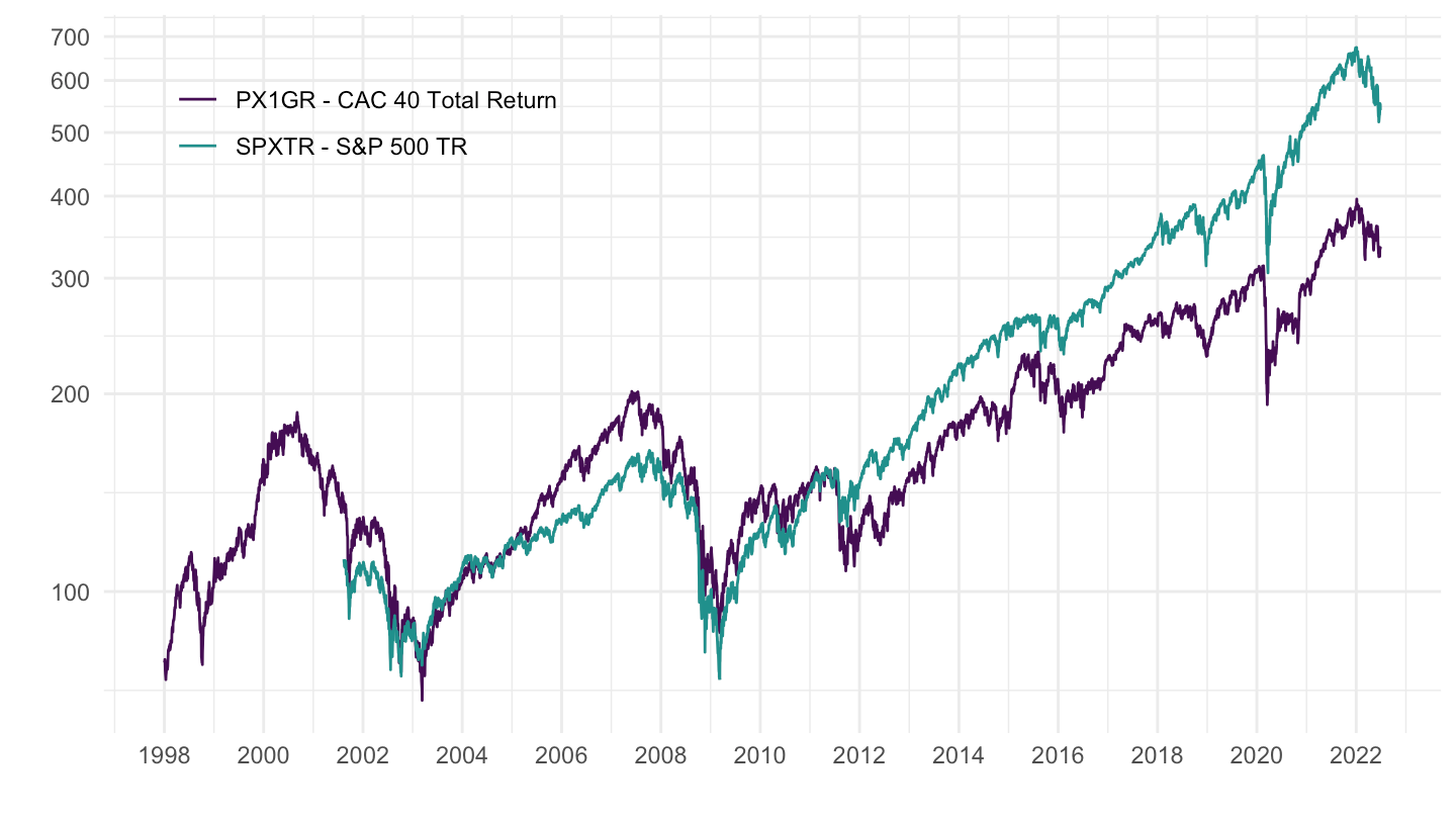
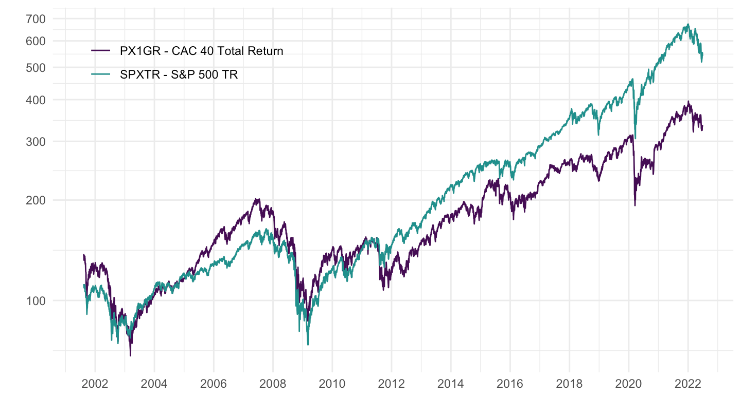
indices %>%
  filter(symbol %in% c("PX1GR", "SPXTR")) %>%
  left_join(indices_var, by = "symbol") %>%
  group_by(symbol) %>%
  filter(Date >= as.Date("2001-08-13")) %>%
  mutate(Close = 100*Close / Close[Date == as.Date("2003-09-04")],
         name = gsub("Gross TR", "Total Return", name)) %>%
  arrange(desc(Date)) %>%
  ggplot + geom_line(aes(x = Date, y = Close, color = paste(symbol, "-", name))) +
  theme_minimal() + xlab("") + ylab("") +
  scale_x_date(breaks = seq(1960, 2022, 2) %>% paste0("-01-01") %>% as.Date,
               labels = date_format("%Y")) +
  scale_y_log10(breaks = seq(100, 20000, 100)) +
  scale_color_manual(values = viridis(3)[1:2]) +
  theme(legend.position = c(0.2, 0.85),
        legend.title = element_blank())