Last data update: 17 sept. 2026, 21:37
Last compile: 10 oct. 2026, 01:12
fig1 |>
  mutate(decile = factor(decile, levels = c("D1", "D5 (médiane)", "D9"))) |>
  ggplot(aes(x = annee, y = indice, color = redistribution)) +
  geom_hline(yintercept = 100, color = "grey60", linewidth = 0.4) +
  geom_line(linewidth = 1) +
  facet_wrap(~ decile) +
  scale_color_manual(values = couleurs_redistribution, name = NULL) +
  theme_minimal(base_size = 13) +
  labs(x = NULL, y = NULL,
       title = "Déciles de niveau de vie (D1, médiane, D9) de 1996 à 2024",
       subtitle = "indice base 100 en 2008, en euros constants (déflaté IPC)") +
  theme(legend.position = "bottom",
        panel.grid.minor = element_blank())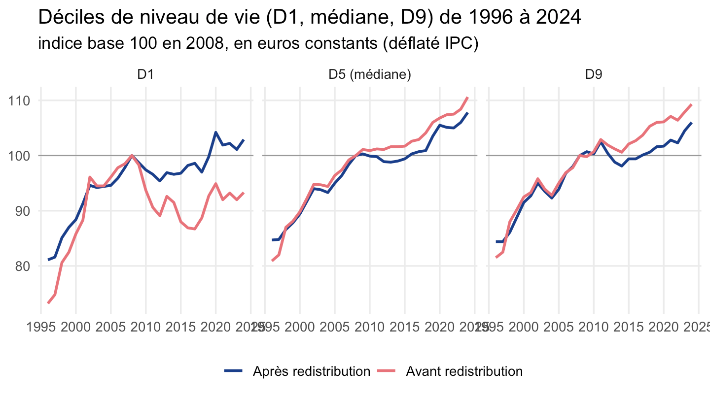
L’Insee déflate ces indices par l’IPC (indice des prix à la consommation). L’IPCH (indice des prix à la consommation harmonisé, utilisé par Eurostat pour les comparaisons européennes) a légèrement plus augmenté depuis 2008 – reconvertir change donc un peu le niveau des courbes, sans changer leur allure générale.
# Ratio IPC/IPCH rebasé à 1 en 2008 (année de référence des indices Insee) :
# multiplier un indice déflaté-IPC par ce ratio le reconvertit en indice
# déflaté-IPCH, sans autre hypothèse.
ratio_ipch <- ipch_ipc |>
  mutate(annee = as.integer(format(date, "%Y"))) |>
  select(annee, INDICATEUR, OBS_VALUE) |>
  pivot_wider(names_from = INDICATEUR, values_from = OBS_VALUE) |>
  transmute(annee, ratio_rebase = (IPC / IPCH) / (IPC[annee == 2008] / IPCH[annee == 2008]))

fig1_deflateurs <- bind_rows(
  fig1 |> mutate(deflateur = "IPC (Insee, original)"),
  fig1 |>
    left_join(ratio_ipch, by = "annee") |>
    mutate(indice = indice * ratio_rebase, deflateur = "IPCH") |>
    select(-ratio_rebase)
)

fig1_deflateurs |>
  mutate(decile = factor(decile, levels = c("D1", "D5 (médiane)", "D9"))) |>
  ggplot(aes(x = annee, y = indice, color = redistribution, linetype = deflateur)) +
  geom_hline(yintercept = 100, color = "grey60", linewidth = 0.4) +
  geom_line(linewidth = 0.9) +
  facet_wrap(~ decile) +
  scale_color_manual(values = couleurs_redistribution, name = NULL) +
  scale_linetype_manual(values = c("IPC (Insee, original)" = "solid", "IPCH" = "22"), name = "Déflateur") +
  theme_minimal(base_size = 13) +
  labs(x = NULL, y = NULL,
       title = "Déciles de niveau de vie, déflatés par l'IPC ou par l'IPCH",
       subtitle = "indice base 100 en 2008, en euros constants") +
  theme(legend.position = "bottom",
        legend.box = "vertical",
        panel.grid.minor = element_blank())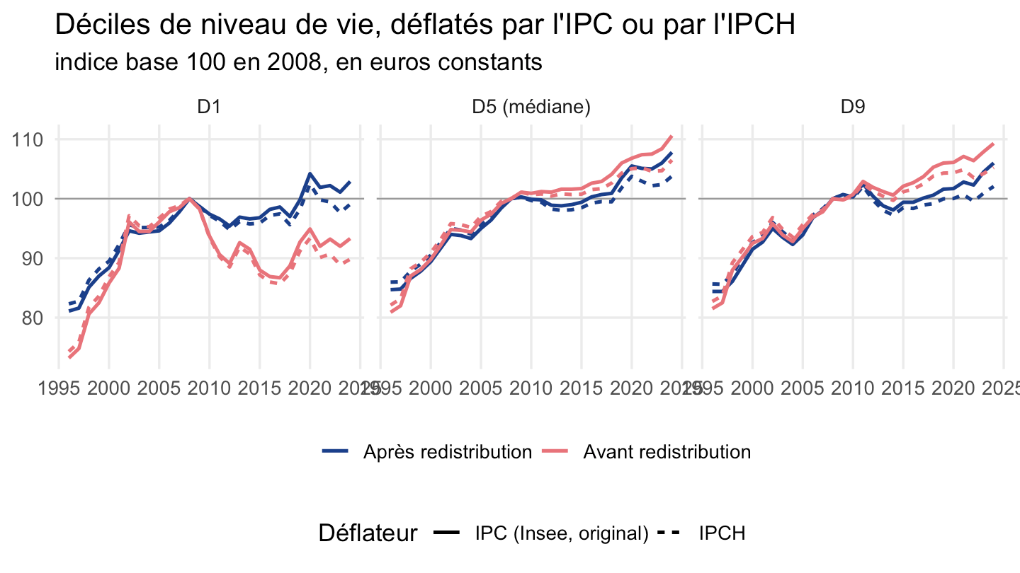
fig2 |>
  rename(`Rapport interdécile D9/D1` = d9_d1,
         `Rapport (100-S80)/S20` = ratio_100s80_s20,
         `Indice de Gini` = gini) |>
  pivot_longer(-annee, names_to = "indicateur", values_to = "valeur") |>
  ggplot(aes(x = annee, y = valeur)) +
  geom_line(linewidth = 1, color = "#1B3F8B") +
  facet_wrap(~ indicateur, scales = "free_y") +
  theme_minimal(base_size = 13) +
  labs(x = NULL, y = NULL,
       title = "Indicateurs d'inégalités de niveau de vie de 1996 à 2024") +
  theme(panel.grid.minor = element_blank())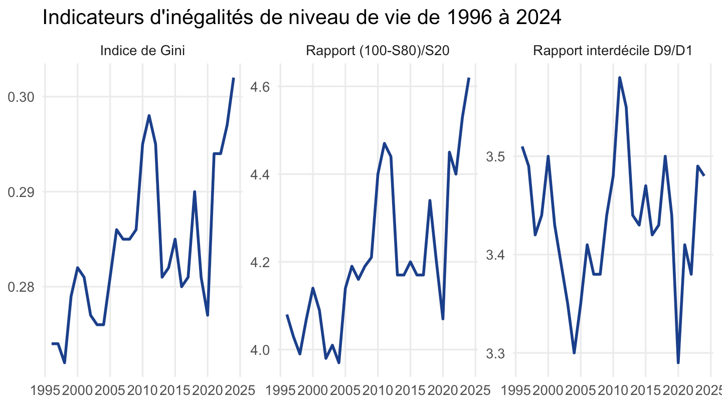
fig3 |>
  filter(str_starts(indicateur, "Taux de pauvreté")) |>
  ggplot(aes(x = annee, y = value)) +
  geom_col(fill = "#1B3F8B") +
  geom_text(aes(label = value), vjust = -0.4, size = 3.5) +
  scale_x_continuous(breaks = 2017:2024) +
  theme_minimal(base_size = 13) +
  labs(x = NULL, y = NULL,
       title = "Taux de pauvreté au seuil de 60 % du niveau de vie médian",
       subtitle = "en % de la population, France métropolitaine") +
  theme(panel.grid.minor = element_blank(),
        panel.grid.major.x = element_blank())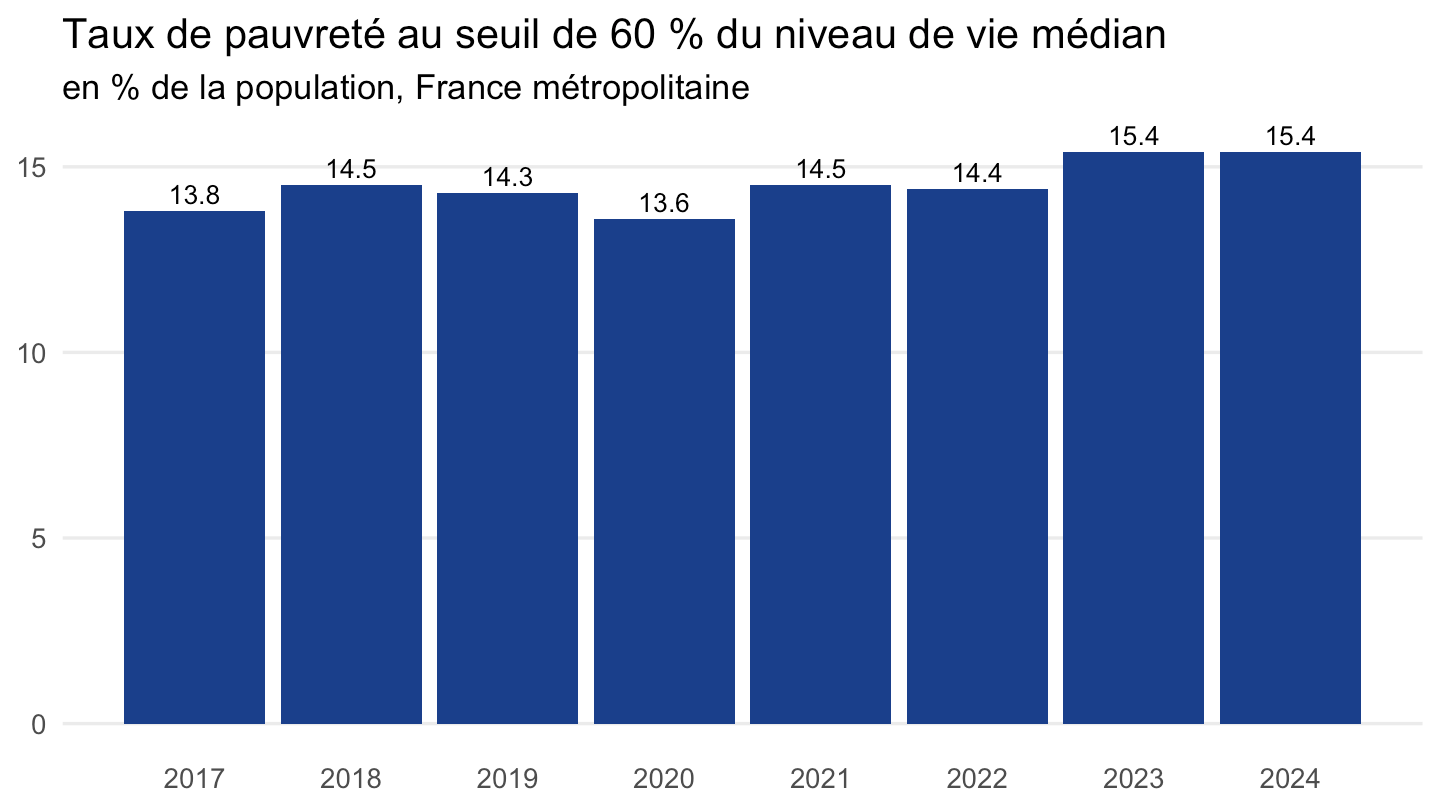
tc3 |>
  filter(indicateur == "Taux de pauvreté (en %)") |>
  ggplot(aes(x = annee, y = value, color = seuil)) +
  geom_line(linewidth = 1) +
  scale_color_manual(values = c("60 % de la médiane" = "#1B3F8B", "50 % de la médiane" = "#E8737A"),
                      name = "Seuil de pauvreté") +
  theme_minimal(base_size = 13) +
  labs(x = NULL, y = NULL,
       title = "Taux de pauvreté de 1996 à 2024",
       subtitle = "aux seuils de 60 % et 50 % du niveau de vie médian (en %)") +
  theme(legend.position = "bottom",
        panel.grid.minor = element_blank())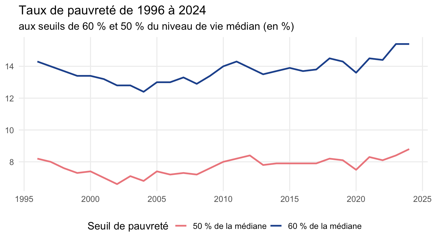
fig4 |>
  filter(section == "Statut d’activité", categorie != "Actifs de 18 ans ou plus",
         categorie != "Inactifs de 18 ans ou plus") |>
  mutate(categorie = fct_reorder(categorie, taux_pauvrete),
         annee = factor(annee)) |>
  ggplot(aes(x = categorie, y = taux_pauvrete, fill = annee)) +
  geom_col(position = position_dodge(width = 0.75), width = 0.7) +
  coord_flip() +
  scale_fill_manual(values = c("2023" = "#8FB0DE", "2024" = "#1B3F8B"), name = NULL) +
  theme_minimal(base_size = 13) +
  labs(x = NULL, y = NULL,
       title = "Taux de pauvreté selon le statut d'activité",
       subtitle = "en 2023 et 2024 (en %)") +
  theme(legend.position = "bottom",
        panel.grid.minor = element_blank(),
        panel.grid.major.y = element_blank())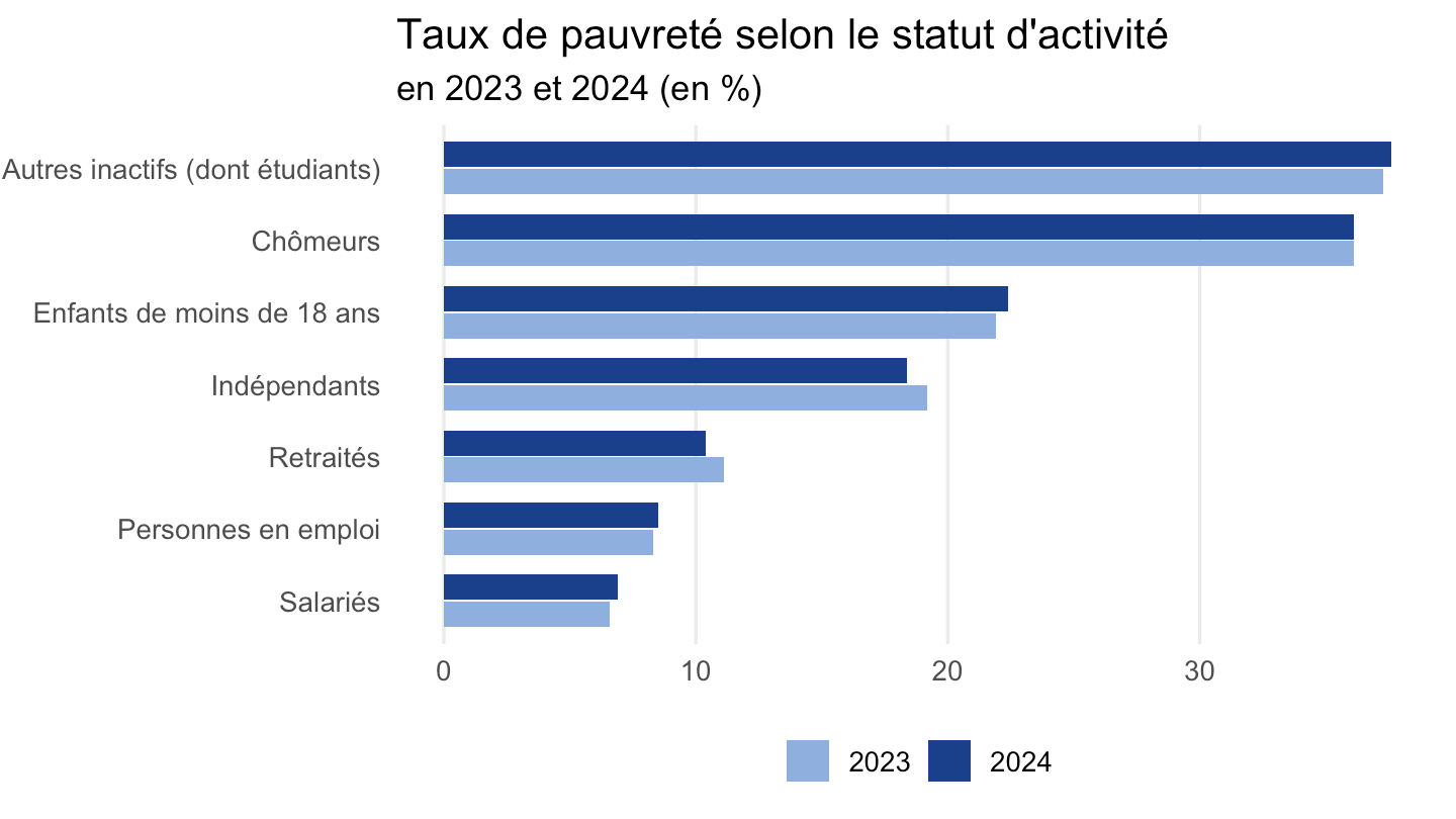
fig4 |>
  filter(section == "Composition du ménage",
         !categorie %in% c("Ensemble", "Personne de référence de moins de 65 ans",
                            "Personne de référence de 65 ans ou plus")) |>
  mutate(categorie = fct_reorder(categorie, taux_pauvrete),
         annee = factor(annee)) |>
  ggplot(aes(x = categorie, y = taux_pauvrete, fill = annee)) +
  geom_col(position = position_dodge(width = 0.75), width = 0.7) +
  facet_wrap(~ groupe_age, scales = "free_y", ncol = 1) +
  coord_flip() +
  scale_fill_manual(values = c("2023" = "#8FB0DE", "2024" = "#1B3F8B"), name = NULL) +
  theme_minimal(base_size = 13) +
  labs(x = NULL, y = NULL,
       title = "Taux de pauvreté selon la composition du ménage",
       subtitle = "en 2023 et 2024 (en %)") +
  theme(legend.position = "bottom",
        panel.grid.minor = element_blank(),
        panel.grid.major.y = element_blank())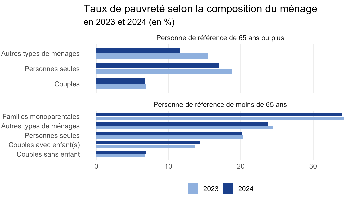
tc1 |>
  mutate(decile = factor(decile, levels = deciles_levels)) |>
  ggplot(aes(x = annee, y = indice, color = decile)) +
  geom_hline(yintercept = 100, color = "grey60", linewidth = 0.4) +
  geom_line(linewidth = 0.9) +
  facet_wrap(~ redistribution) +
  scale_color_viridis_d(name = "Décile") +
  theme_minimal(base_size = 13) +
  labs(x = NULL, y = NULL,
       title = "Éventail des déciles de niveau de vie (D1 à D9) de 1996 à 2024",
       subtitle = "indice base 100 en 2008, en euros constants") +
  theme(legend.position = "bottom",
        panel.grid.minor = element_blank())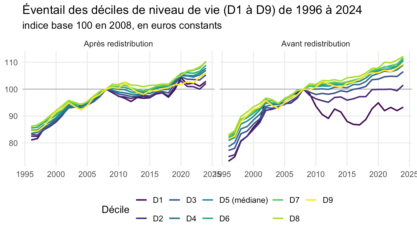
tc2 |>
  pivot_wider(names_from = annee, values_from = value) |>
  arrange(redistribution, indicateur) |>
  gt(groupname_col = "redistribution") |>
  tab_header(title = "Niveaux de vie et indicateurs d'inégalités de 1996 à 2024") |>
  fmt_number(columns = where(is.numeric), decimals = 1) |>
  cols_label(indicateur = "") |>
  opt_interactive(use_search = TRUE, use_pagination = FALSE, use_compact_mode = TRUE,
                   use_resizers = TRUE, use_highlight = TRUE) |>
tab_options(table.width = "100%")tc4 |>
filter(niveau_densite != "Ensemble") |>
mutate(niveau_densite = fct_reorder(niveau_densite, taux_pauvrete),
annee = factor(annee)) |>
ggplot(aes(x = niveau_densite, y = taux_pauvrete, fill = annee)) +
geom_col(position = position_dodge(width = 0.75), width = 0.7) +
coord_flip() +
scale_fill_manual(values = c("2023" = "#8FB0DE", "2024" = "#1B3F8B"), name = NULL) +
theme_minimal(base_size = 13) +
labs(x = NULL, y = NULL,
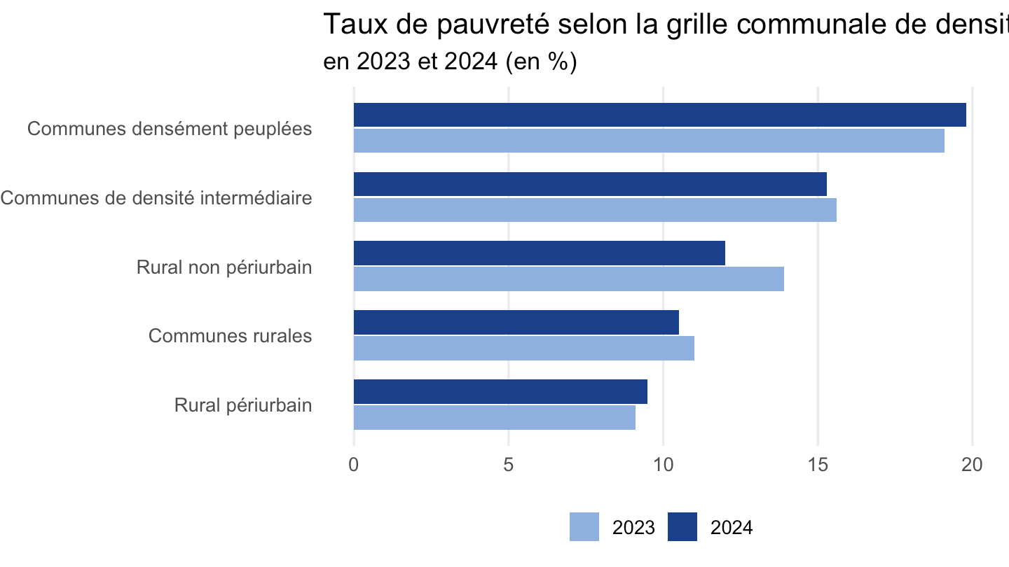
title = "Taux de pauvreté selon la grille communale de densité",
subtitle = "en 2023 et 2024 (en %)") +
theme(legend.position = "bottom",
panel.grid.minor = element_blank(),
panel.grid.major.y = element_blank())