ip1863_fig3 %>%
mutate(salaires_min = 1100 + 100*seq(0, 76, 1),
salaires_min = ifelse(salaires_min == 1100, 0, salaires_min),
salaires_max = 1200 + 100*seq(0, 76, 1),
salaires_max = ifelse(salaires_max == 8800, Inf, salaires_max)) %>%
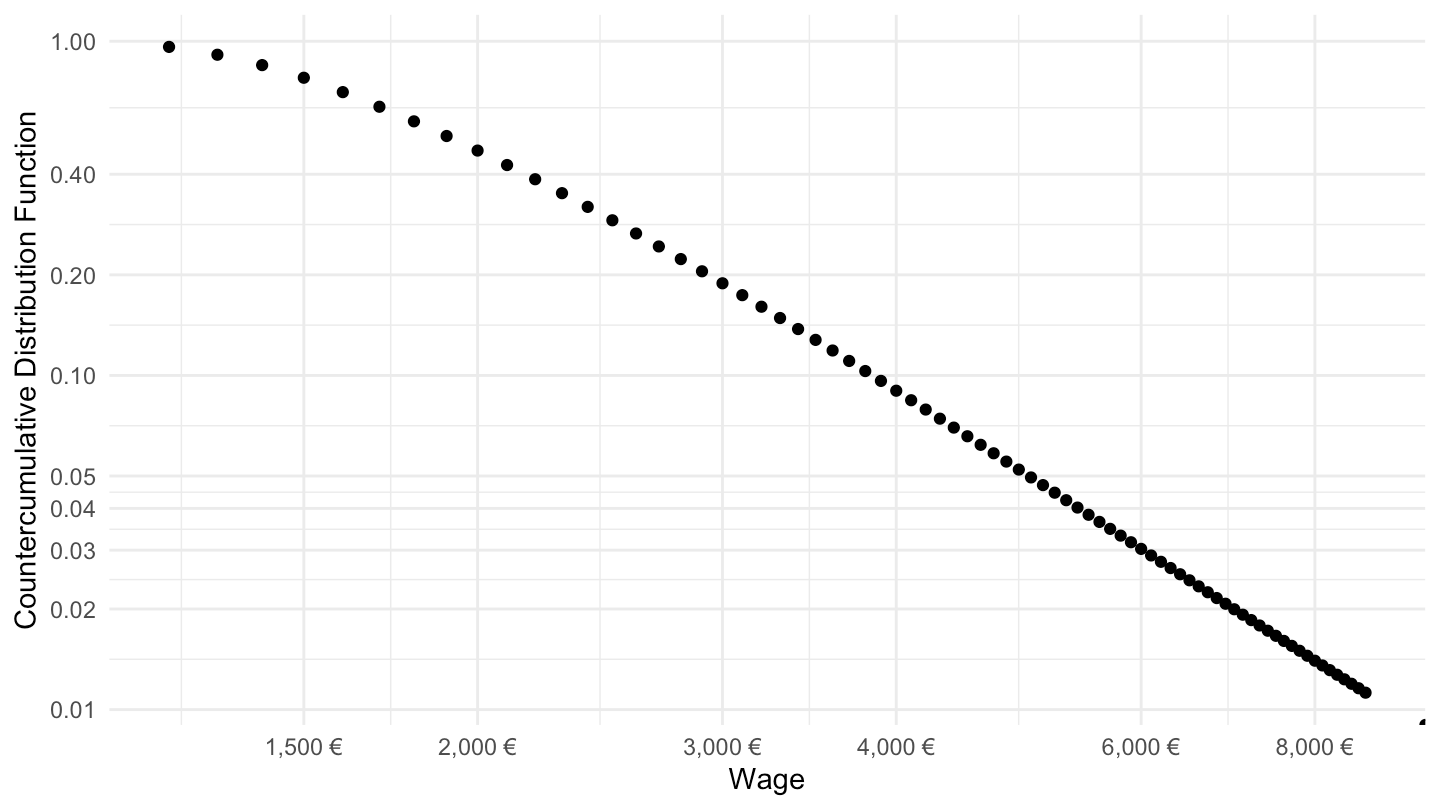
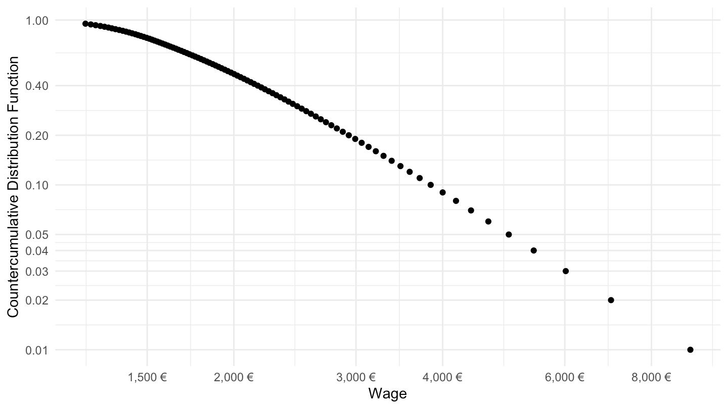
mutate(effectifs_cum = 1 - cumsum(effectifs)/sum(effectifs)) %>%
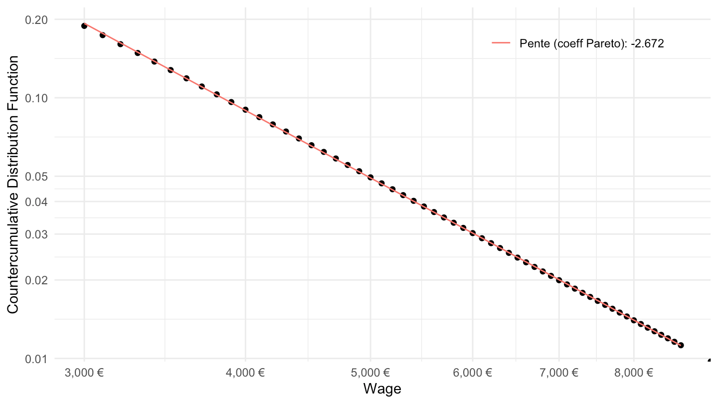
filter(effectifs_cum <= 0.2) %>%
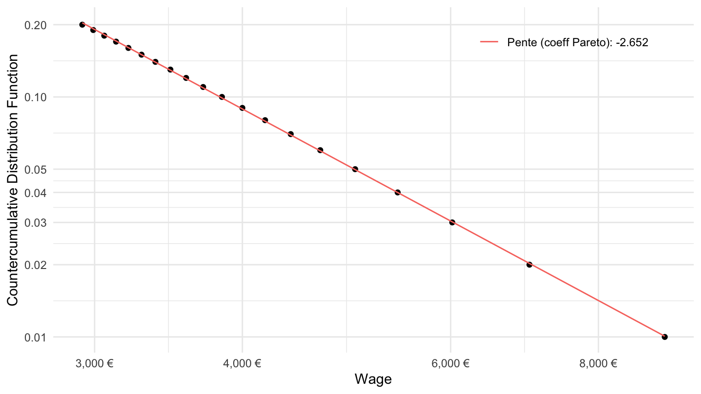
ggplot(.) + theme_minimal() + xlab("Wage") + ylab("Countercumulative Distribution Function") +
geom_point(aes(x = salaires_max, y = effectifs_cum)) +
scale_x_log10(breaks = c(1000, 1500, 2000, 3000, 4000, 5000, 6000, 7000, 8000),
labels = dollar_format(prefix = "", accuracy = 1, suffix = " €")) +
scale_y_log10(breaks = c(seq(0.01, 0.05, 0.01), 0.1, 0.2, 0.4, 1)) +
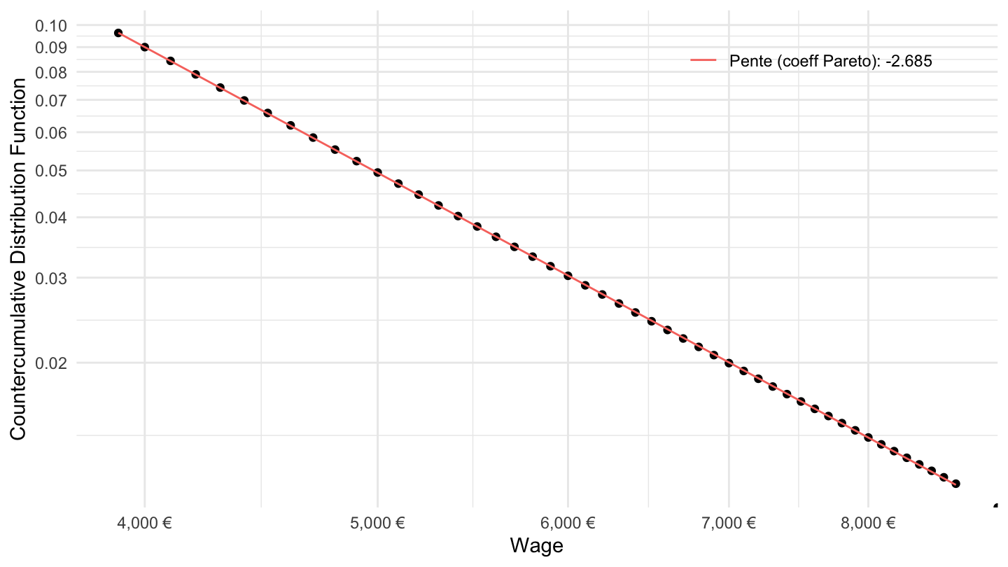
geom_function(aes(colour = paste0("Pente (coeff Pareto): ", round(fit1$coefficients[2],3))), fun = function(x) exp(fit1$coefficients[1] + fit1$coefficients[2]*log(x))) +
theme(legend.position = c(0.8, 0.9),
legend.title = element_blank())