Last data update: 29 sept. 2026, 21:16
Last compile: 19 oct. 2026, 02:10
g1 |>
  ggplot(aes(x = annee, y = valeur / 100, color = zone)) +
  geom_line(linewidth = 1) +
  geom_point() +
  geom_hline(yintercept = 0, color = "grey30") +
  scale_y_continuous(labels = scales::percent_format(accuracy = 1)) +
  scale_color_brewer(palette = "Set1", name = NULL) +
  theme_minimal(base_size = 11) +
  labs(x = NULL, y = NULL,
       title = "Variations annuelles des prix des appartements anciens",
       subtitle = "Île-de-France, par zone") +
  theme(legend.position = "bottom", panel.grid.minor = element_blank())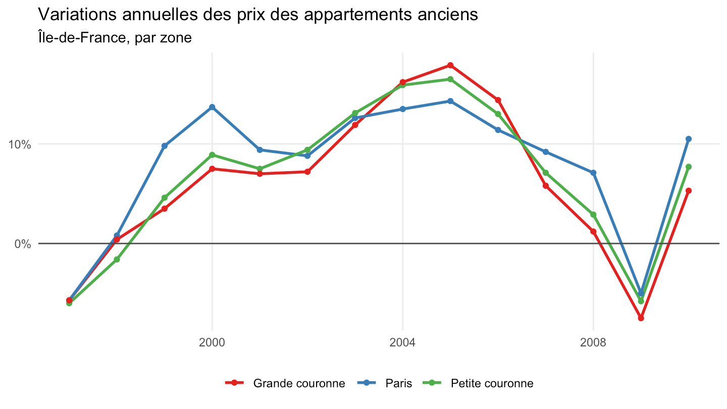
g2 |>
  ggplot(aes(x = annee, y = valeur, color = indicateur)) +
  geom_line(linewidth = 1) +
  scale_color_brewer(palette = "Set1", name = NULL) +
  theme_minimal(base_size = 9) +
  labs(x = NULL, y = "Base 100 en 2000",
       title = "Prix à la consommation, loyers, prix des logements anciens et revenus",
       subtitle = "France, indice base 100 en 2000") +
  theme(legend.position = "bottom", panel.grid.minor = element_blank()) +
  guides(color = guide_legend(ncol = 2))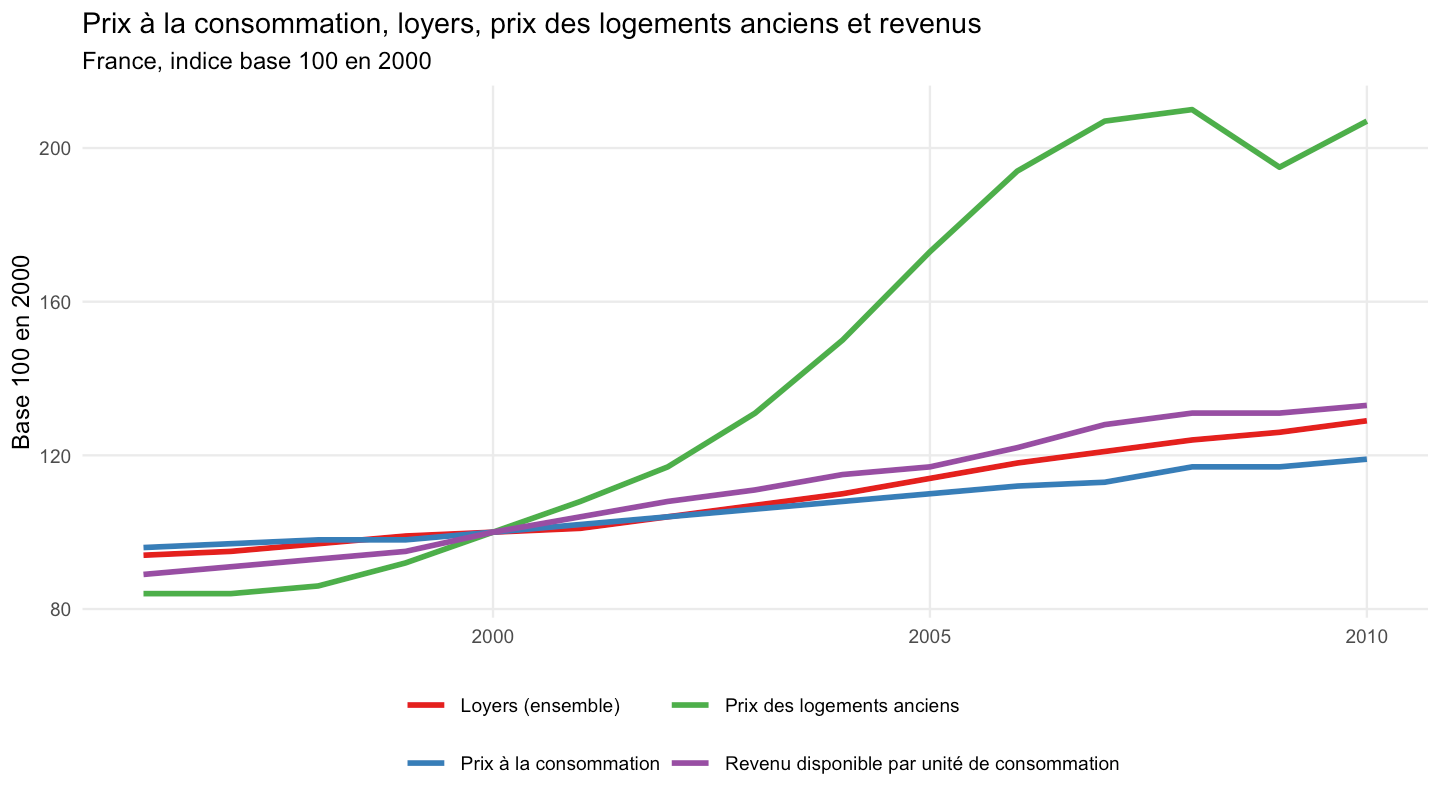
g3 |>
  ggplot(aes(x = annee, y = valeur / 100, color = indicateur)) +
  geom_line(linewidth = 1) +
  geom_point() +
  scale_y_continuous(labels = scales::percent_format(accuracy = 0.1)) +
  scale_color_brewer(palette = "Set1", name = NULL) +
  theme_minimal(base_size = 11) +
  labs(x = NULL, y = NULL,
       title = "Variations annuelles des loyers",
       subtitle = "HLM, secteur libre, prix à la consommation") +
  theme(legend.position = "bottom", panel.grid.minor = element_blank())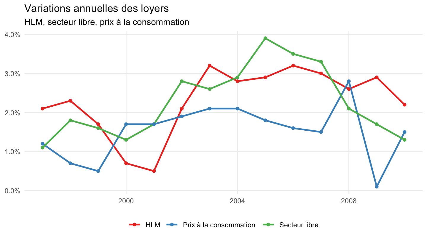
g4 |>
  mutate(serie = paste(secteur, zone, sep = " - ")) |>
  ggplot(aes(x = annee, y = valeur, color = serie)) +
  geom_line(linewidth = 1) +
  scale_color_brewer(palette = "Set2", name = NULL) +
  theme_minimal(base_size = 9) +
  labs(x = NULL, y = "Base 100 en 2000",
       title = "Indices de loyers HLM et secteur libre",
       subtitle = "province et agglomération parisienne") +
  theme(legend.position = "bottom", panel.grid.minor = element_blank()) +
  guides(color = guide_legend(ncol = 2))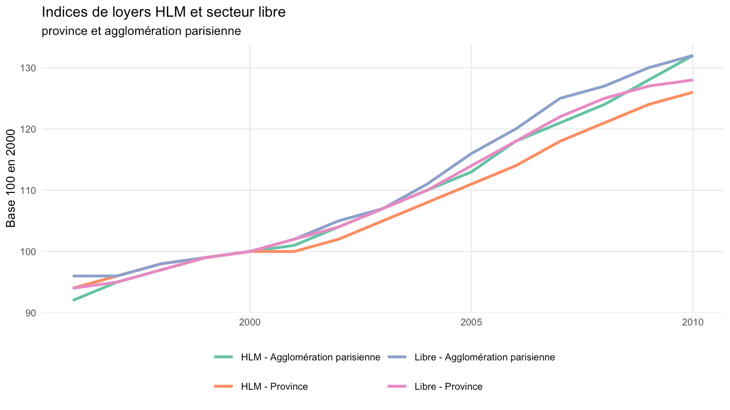
t1 |>
  filter(zone == "Île-de-France") |>
  mutate(statut = fct_reorder(statut, valeur)) |>
  ggplot(aes(x = statut, y = valeur / 100, fill = factor(annee))) +
  geom_col(position = "dodge") +
  coord_flip() +
  scale_y_continuous(labels = scales::percent_format(accuracy = 1)) +
  scale_fill_manual(values = c("#1B3F8B", "#E8737A"), name = NULL) +
  theme_minimal(base_size = 10) +
  labs(x = NULL, y = NULL,
       title = "Taux d'effort médian par statut d'occupation",
       subtitle = "Île-de-France, 1996 vs. 2006") +
  theme(legend.position = "bottom", panel.grid.minor = element_blank())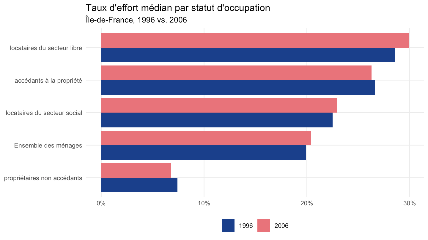
t1 |>
  filter(statut == "Ensemble des ménages") |>
  ggplot(aes(x = zone, y = valeur / 100, fill = factor(annee))) +
  geom_col(position = "dodge") +
  scale_y_continuous(labels = scales::percent_format(accuracy = 1)) +
  scale_fill_manual(values = c("#1B3F8B", "#E8737A"), name = NULL) +
  theme_minimal(base_size = 11) +
  labs(x = NULL, y = NULL,
       title = "Taux d'effort médian de l'ensemble des ménages",
       subtitle = "par zone, 1996 vs. 2006") +
  theme(legend.position = "bottom", panel.grid.minor = element_blank())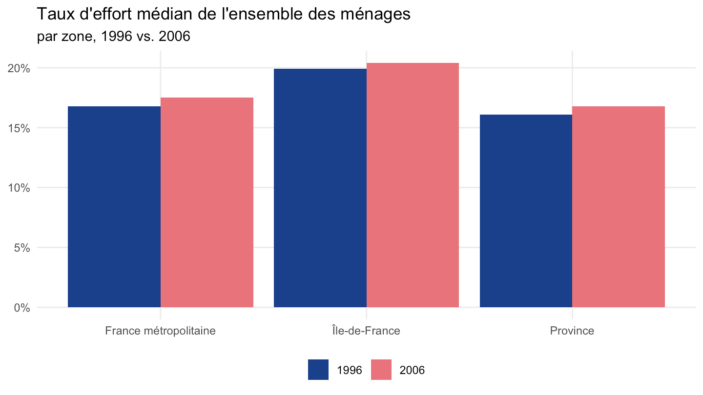
t2 |>
  filter(groupe == "Localisation") |>
  mutate(critere = fct_reorder(critere, valeur)) |>
  ggplot(aes(x = critere, y = valeur / 100, fill = factor(annee))) +
  geom_col(position = "dodge") +
  coord_flip() +
  scale_y_continuous(labels = scales::percent_format(accuracy = 1)) +
  scale_fill_manual(values = c("#1B3F8B", "#E8737A"), name = NULL) +
  theme_minimal(base_size = 9) +
  labs(x = NULL, y = NULL,
       title = "Rapport médian entre le loyer annuel et le prix",
       subtitle = "par localisation, 1996 vs. 2006") +
  theme(legend.position = "bottom", panel.grid.minor = element_blank())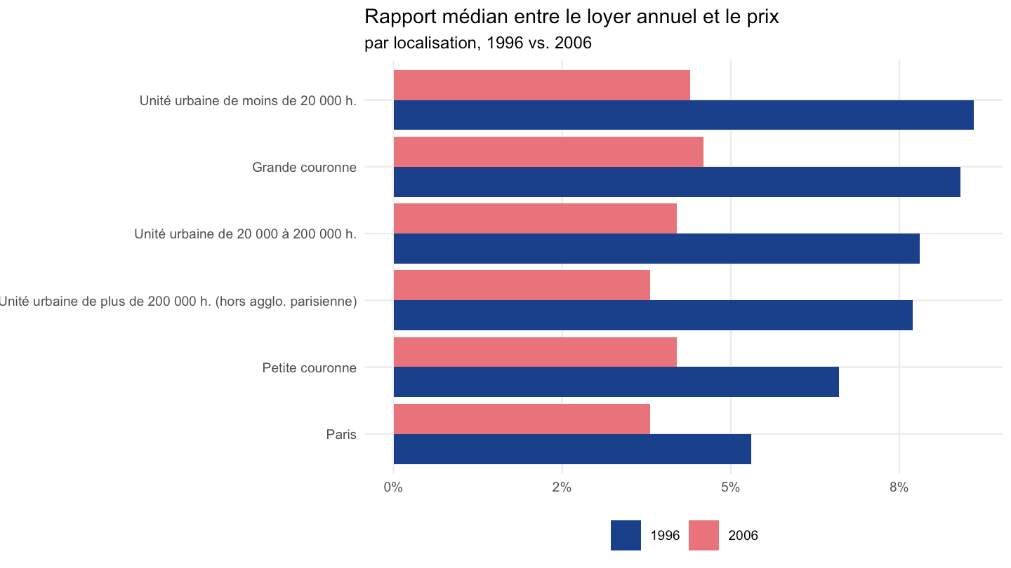
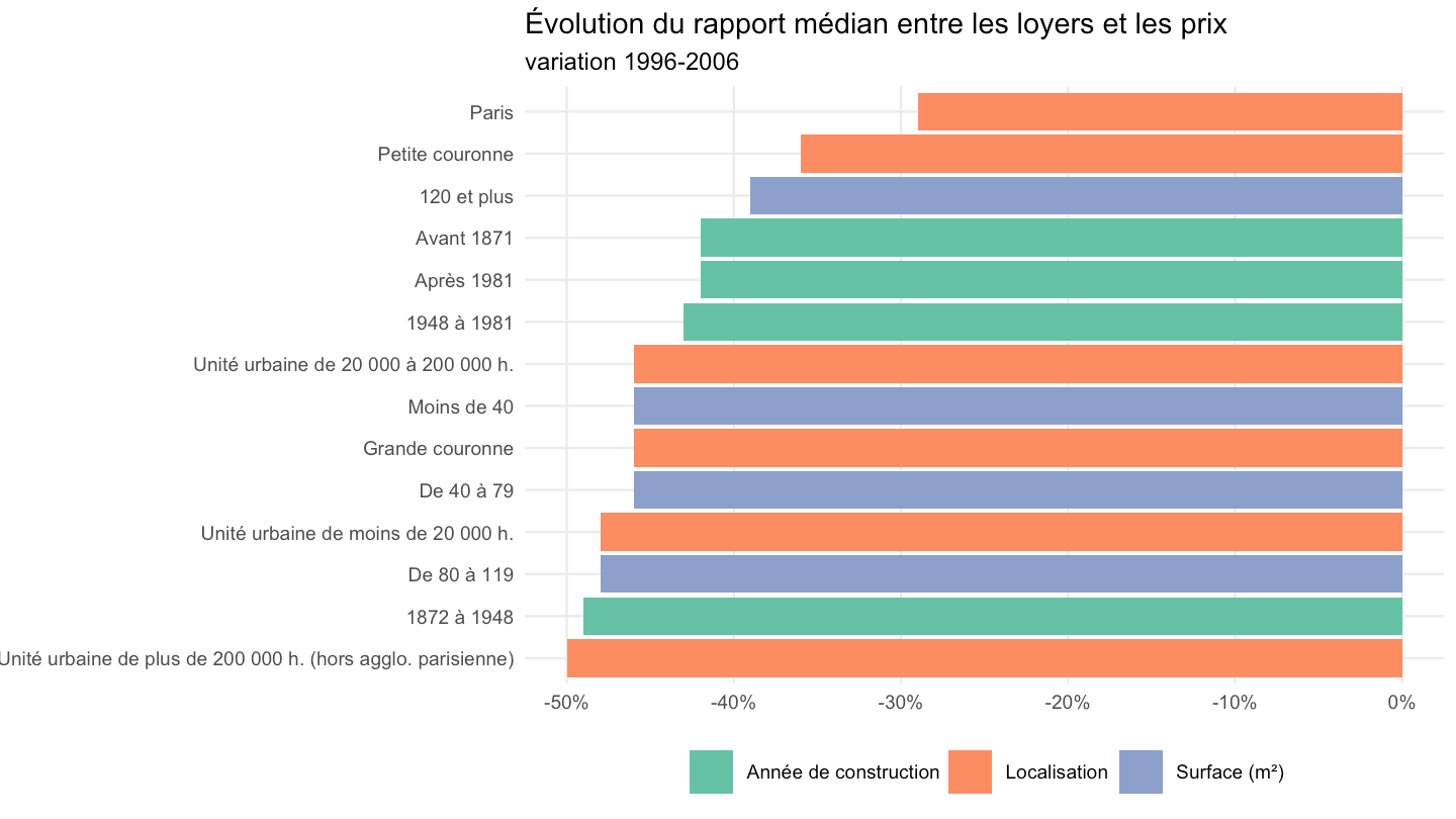
t2 |>
  distinct(critere, variation, groupe) |>
  filter(groupe != "Ensemble") |>
  mutate(critere = fct_reorder(critere, variation)) |>
  ggplot(aes(x = critere, y = variation / 100, fill = groupe)) +
  geom_col() +
  coord_flip() +
  scale_y_continuous(labels = scales::percent_format(accuracy = 1)) +
  scale_fill_brewer(palette = "Set2", name = NULL) +
  theme_minimal(base_size = 9) +
  labs(x = NULL, y = NULL,
       title = "Évolution du rapport médian entre les loyers et les prix",
       subtitle = "variation 1996-2006") +
  theme(legend.position = "bottom", panel.grid.minor = element_blank())