Code
i_g("bib/insee/FPORSOC22/F29/table2.png")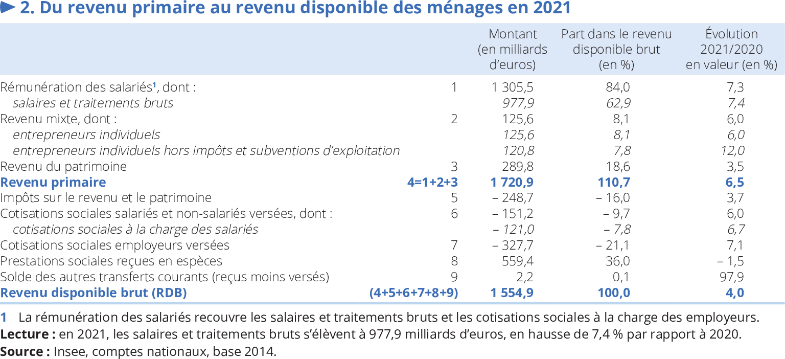
Données - INSEE
i_g("bib/insee/FPORSOC22/F29/table2.png")
i_g("bib/insee/FPS2021/revenu-primaire-RDB.png")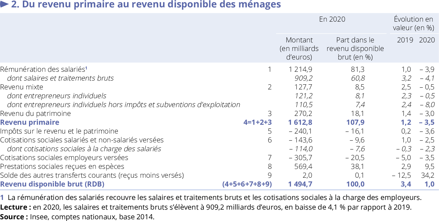

« Mesurer “le” pouvoir d’achat », F. Geerolf, 9 juillet 2024. [ html] [ pdf] [ handouts] [ slides] [ slides] [ github]
« La taxe inflationniste, le pouvoir d’achat, le taux d’épargne et le déficit public », F. Geerolf, 9 juillet 2024. [ html] [ pdf] [ handouts] [ slides] [ slides] [ github]
« Inflation en France : IPC ou IPCH ? », F. Geerolf, 9 juillet 2024. [ html] [ pdf] [ handouts] [ slides] [ slides] [ github]
T_2101 %>%
  group_by(line, variable, Variable) %>%
  summarise(Nobs = n()) %>%
print_table_conditional| line | variable | Variable | Nobs |
|---|---|---|---|
| 1 | D11 | Salaires et traitements bruts | 66 |
| 2 | D613CE | Cotisations sociales effectives obligatoires à la charge des salariés | 66 |
| 3 | D11X613CE | Salaires et traitements nets | 66 |
| 4 | D62 | Prestations sociales autres que transferts sociaux en nature | 66 |
| 5 | RSS | Revenus salariaux et sociaux | 66 |
| 6 | B2A3G | Excédent brut d’exploitation et revenu mixte brut | 66 |
| 7 | D613NSI | Cotisations des non salariés | 66 |
| 8 | B6G | Revenu disponible brut | 66 |
| 9 | B6G | Revenu disponible brut | 66 |
| 10 | P31 | Dépense de consommation individuelle - indice du prix de la consommation des ménages | 66 |
| 11 | _PAM | Pouvoir d’achat du rdb des ménages (**) | 65 |
| 12 | _PAM_PERSONNE | Pouvoir d’achat du rdb par personne | 65 |
| 13 | _PAM_MENAGE | Pouvoir d’achat du rdb par ménage | 65 |
| 14 | _PAM_UC | Pouvoir d’achat du rdb par unité de consommation | 65 |
| 15 | POP | Population | 66 |
| 16 | MENF | Moyenne annuelle du nombre de ménages en France entière | 66 |
| 17 | UC | Unités de consommation | 66 |
T_2101 %>%
  filter(year %in% c("2017", "2024")) %>%
  spread(year, value) %>%
  mutate(croissance = round(100*(`2024`/`2017`-1), 2)) %>%
  arrange(desc(croissance)) %>%
print_table_conditional()| variable | Variable | line | 2017 | 2024 | croissance |
|---|---|---|---|---|---|
| P31 | Dépense de consommation individuelle - indice du prix de la consommation des ménages | 10 | 0.767 | 2.187 | 185.14 |
| _PAM_MENAGE | Pouvoir d’achat du rdb par ménage | 13 | 0.829 | 1.671 | 101.57 |
| B6G | Revenu disponible brut | 9 | 2.501 | 4.801 | 91.96 |
| _PAM_UC | Pouvoir d’achat du rdb par unité de consommation | 14 | 1.163 | 2.068 | 77.82 |
| _PAM_PERSONNE | Pouvoir d’achat du rdb par personne | 12 | 1.314 | 2.289 | 74.20 |
| _PAM | Pouvoir d’achat du rdb des ménages (**) | 11 | 1.720 | 2.557 | 48.66 |
| B6G | Revenu disponible brut | 8 | 1387.380 | 1861.088 | 34.14 |
| D11X613CE | Salaires et traitements nets | 3 | 760.073 | 997.125 | 31.19 |
| B2A3G | Excédent brut d’exploitation et revenu mixte brut | 6 | 311.645 | 406.978 | 30.59 |
| RSS | Revenus salariaux et sociaux | 5 | 1256.715 | 1628.351 | 29.57 |
| D11 | Salaires et traitements bruts | 1 | 880.657 | 1134.133 | 28.78 |
| D62 | Prestations sociales autres que transferts sociaux en nature | 4 | 496.642 | 631.226 | 27.10 |
| D613NSI | Cotisations des non salariés | 7 | 29.549 | 36.307 | 22.87 |
| D613CE | Cotisations sociales effectives obligatoires à la charge des salariés | 2 | 120.584 | 137.008 | 13.62 |
| MENF | Moyenne annuelle du nombre de ménages en France entière | 16 | 0.884 | 0.871 | -1.47 |
| UC | Unités de consommation | 17 | 0.550 | 0.479 | -12.91 |
| POP | Population | 15 | 0.401 | 0.262 | -34.66 |
T_2101 %>%
  filter(line %in% c(1, 3)) %>%
  left_join(gdp, by = "year") %>%
  year_to_date2 %>%
  ggplot + geom_line(aes(x = date, y = value / gdp, color = Variable)) +
  theme_minimal() + xlab("") + ylab("% du PIB") +
  scale_x_date(breaks ="5 years",
               labels = date_format("%Y")) +
  scale_y_continuous(breaks = 0.01*seq(-10, 100, 1),
                     labels = percent_format(accuracy = 1)) +
  theme(legend.position = c(0.2, 0.15),
        legend.title = element_blank())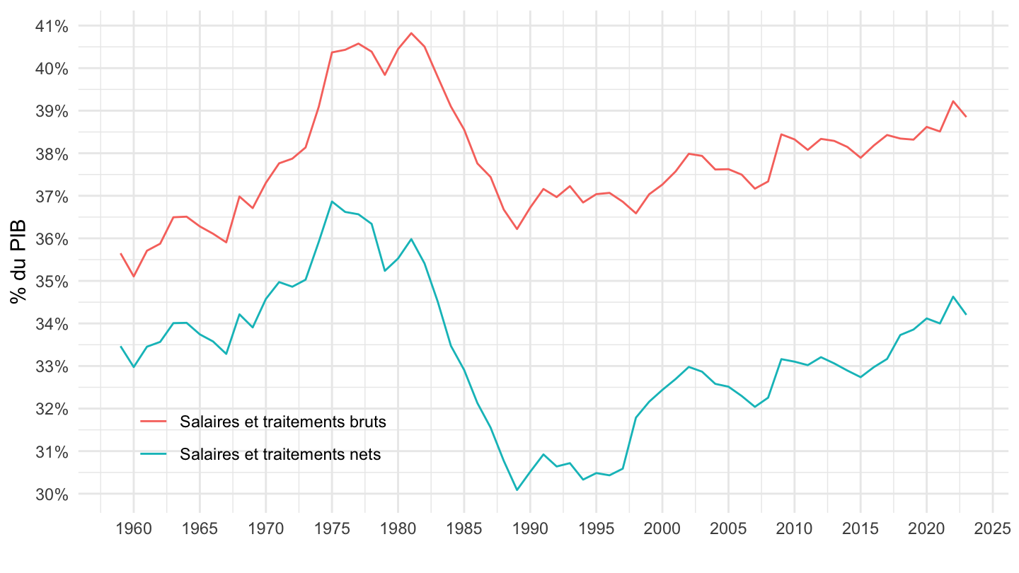
T_2101 %>%
  filter(line %in% c(1, 3)) %>%
  left_join(rdb, by = "year") %>%
  year_to_date2 %>%
  ggplot + geom_line(aes(x = date, y = value / rdb, color = Variable)) +
  theme_minimal() + xlab("") + ylab("% du RDB") +
  scale_x_date(breaks ="5 years",
               labels = date_format("%Y")) +
  scale_y_continuous(breaks = 0.01*seq(-10, 100, 1),
                     labels = percent_format(accuracy = 1)) +
  theme(legend.position = c(0.15, 0.93),
        legend.title = element_blank())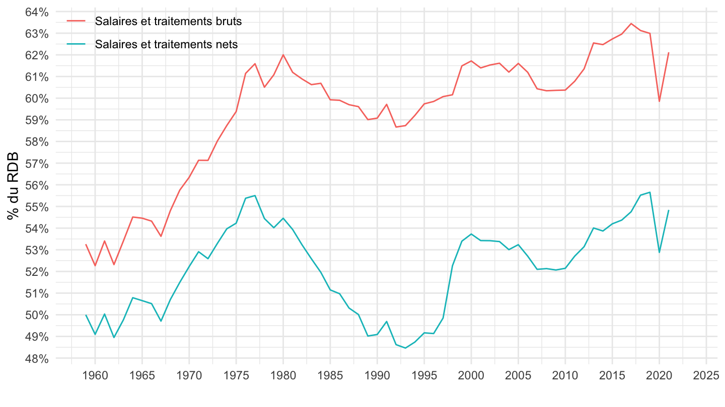
T_2101 %>%
  filter(line %in% c(1, 3)) %>%
  year_to_date2 %>%
  filter(date >= as.Date("2008-01-01")) %>%
  group_by(Variable) %>%
  mutate(value = 100*value/value[1]) %>%
  ggplot + geom_line(aes(x = date, y = value, color = Variable)) +
  theme_minimal() + xlab("") + ylab("Base 100 = 2008") +
  scale_x_date(breaks = as.Date(paste0(seq(1940, 2100, 2), "-01-01")),
               labels = date_format("%Y")) +
  scale_y_log10(breaks = seq(-10, 200, 5)) +
  theme(legend.position = c(0.3, 0.93),
        legend.title = element_blank())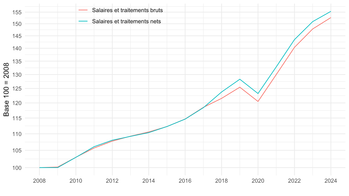
T_2101 %>%
  filter(line %in% c(1, 3)) %>%
  year_to_date2 %>%
  filter(date >= as.Date("2017-01-01")) %>%
  group_by(Variable) %>%
  mutate(value = 100*value/value[1]) %>%
  ggplot + geom_line(aes(x = date, y = value, color = Variable)) +
  theme_minimal() + xlab("") + ylab("Base 100 = 2017") +
  scale_x_date(breaks = as.Date(paste0(seq(1940, 2100, 1), "-01-01")),
               labels = date_format("%Y")) +
  scale_y_log10(breaks = seq(-10, 200, 5)) +
  theme(legend.position = c(0.3, 0.93),
        legend.title = element_blank()) +
  geom_label(data = . %>% filter(date == max(date)),
             aes(x = date, y = value, label = round(value, 1), color = Variable), show.legend = F)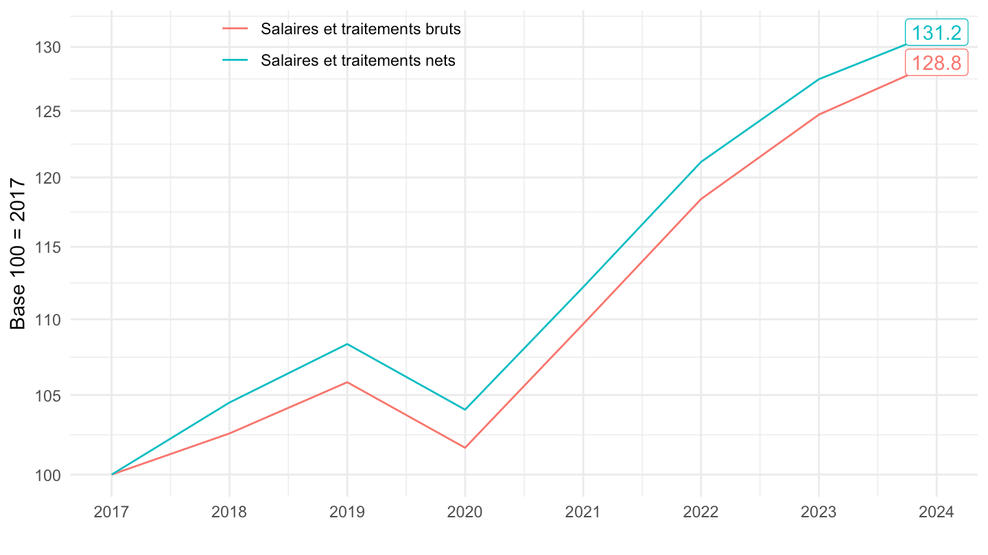
T_2101 %>%
  filter(variable %in% c("D11", "D62")) %>%
  year_to_date2 %>%
  select(date, variable, value) %>%
  spread(variable, value) %>%
  mutate(value = D62/D11) %>%
  ggplot + geom_line(aes(x = date, y = value)) +
  theme_minimal() + xlab("") + ylab("Prestations sociales hors transferts en nature\n% des salaires nets") +
  scale_x_date(breaks ="5 years",
               labels = date_format("%Y")) +
  scale_y_continuous(breaks = 0.01*seq(-10, 100, 2),
                     labels = percent_format(accuracy = 1)) +
  theme(legend.position = c(0.5, 0.9),
        legend.title = element_blank())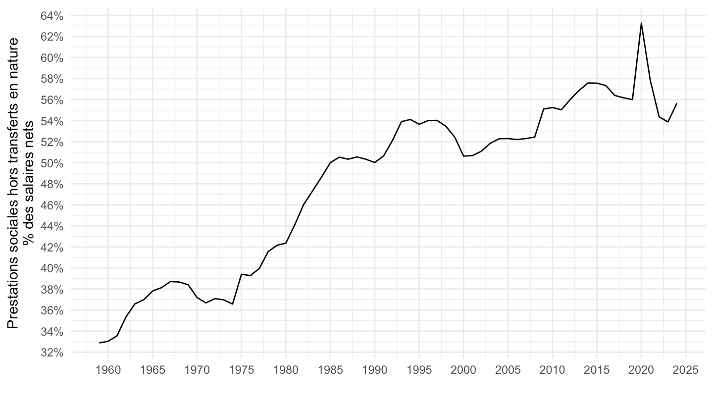
T_2101 %>%
  filter(line %in% c(4, 6)) %>%
  left_join(gdp, by = "year") %>%
  year_to_date2 %>%
  ggplot + geom_line(aes(x = date, y = value / gdp, color = Variable)) +
  theme_minimal() + xlab("") + ylab("% du PIB") +
  scale_x_date(breaks ="5 years",
               labels = date_format("%Y")) +
  scale_y_continuous(breaks = 0.01*seq(-10, 100, 1),
                     labels = percent_format(accuracy = 1)) +
  theme(legend.position = c(0.5, 0.9),
        legend.title = element_blank())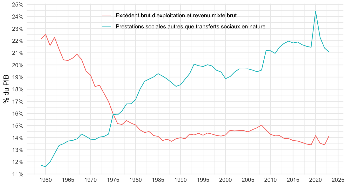
T_2101 %>%
  filter(line %in% c(4, 6)) %>%
  left_join(rdb, by = "year") %>%
  year_to_date2 %>%
  ggplot + geom_line(aes(x = date, y = value / rdb, color = Variable)) +
  theme_minimal() + xlab("") + ylab("% du RDB") +
  scale_x_date(breaks ="5 years",
               labels = date_format("%Y")) +
  scale_y_continuous(breaks = 0.01*seq(-10, 100, 1),
                     labels = percent_format(accuracy = 1)) +
  theme(legend.position = c(0.5, 0.9),
        legend.title = element_blank())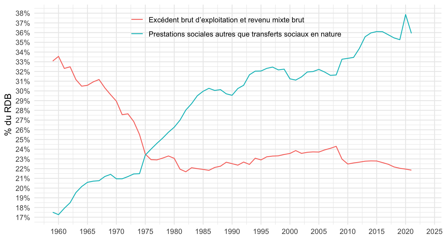
T_2101 %>%
  filter(line %in% c(4, 6)) %>%
  year_to_date2 %>%
  filter(date >= as.Date("2008-01-01")) %>%
  group_by(Variable) %>%
  mutate(value = 100*value/value[1]) %>%
  ggplot + geom_line(aes(x = date, y = value, color = Variable)) +
  theme_minimal() + xlab("") + ylab("Base 100 = 2008") +
  scale_x_date(breaks = as.Date(paste0(seq(1940, 2100, 2), "-01-01")),
               labels = date_format("%Y")) +
  scale_y_log10(breaks = seq(-10, 200, 5)) +
  theme(legend.position = c(0.3, 0.93),
        legend.title = element_blank())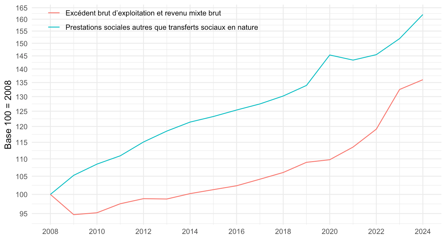
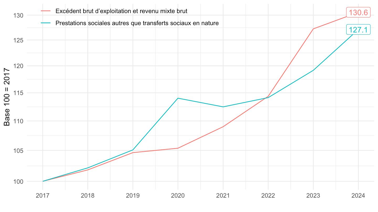
T_2101 %>%
  filter(line %in% c(4, 6)) %>%
  year_to_date2 %>%
  filter(date >= as.Date("2017-01-01")) %>%
  group_by(Variable) %>%
  mutate(value = 100*value/value[1]) %>%
  ggplot + geom_line(aes(x = date, y = value, color = Variable)) +
  theme_minimal() + xlab("") + ylab("Base 100 = 2017") +
  scale_x_date(breaks = as.Date(paste0(seq(1940, 2100, 1), "-01-01")),
               labels = date_format("%Y")) +
  scale_y_log10(breaks = seq(-10, 200, 5)) +
  theme(legend.position = c(0.3, 0.93),
        legend.title = element_blank()) +
  geom_label(data = . %>% filter(date == max(date)),
             aes(x = date, y = value, label = round(value, 1), color = Variable), show.legend = F)