Revenu disponible brut des ménages - T19F054

Données - INSEE

Last data update: 26 oct. 2026, 19:30

Last compile: 26 oct. 2026, 19:33

Revenu disponible brut des ménages

d1 |>
  filter(!is.na(valeur), !is.na(annee), !total100) |>
  ggplot(aes(x = annee, y = valeur, color = cle, group = cle)) +
  geom_line(linewidth = 1.1) +
  geom_point(size = 1.4) +
  scale_color_brewer(palette = "Dark2", name = NULL, labels = scales::label_wrap(45)) +
  theme_pub() +
  labs(x = NULL, y = "en milliards d'euros",
       title = str_wrap("Revenu disponible brut des ménages", 75)) +
  guides(color = guide_legend(ncol = 2))

Évolution du revenu disponible brut et du pouvoir d’achat des ménages

d2 |>
  filter(!is.na(valeur), !total100) |>
  mutate(lab = fct_inorder(libelle), serie = fct_inorder(serie)) |>
  ggplot(aes(x = serie, y = fct_rev(lab), fill = valeur)) +
  geom_tile(color = "white") +
  scale_x_discrete(labels = scales::label_wrap(12), position = "top") +
  scale_y_discrete(labels = scales::label_wrap(40)) +
  scale_fill_gradient(low = "#F4F8FD", high = bleu, name = "en %") +
  theme_pub(9) +
  labs(x = NULL, y = NULL, title = str_wrap("Évolution du revenu disponible brut et du pouvoir d’achat des ménages", 75)) +
  theme(legend.position = "right", panel.grid = element_blank())

Évolution du revenu disponible et du pouvoir d’achat des ménages

d3 |>
  filter(!is.na(valeur), !is.na(annee), !total100) |>
  ggplot(aes(x = annee, y = valeur, color = cle, group = cle)) +
  geom_line(linewidth = 1.1) +
  geom_point(size = 1.4) +
  scale_color_brewer(palette = "Dark2", name = NULL, labels = scales::label_wrap(45)) +
  theme_pub() +
  labs(x = NULL, y = "par rapport à l'année précédente en %",
       title = str_wrap("Évolution du revenu disponible et du pouvoir d’achat des ménages", 75)) +
  guides(color = guide_legend(ncol = 2))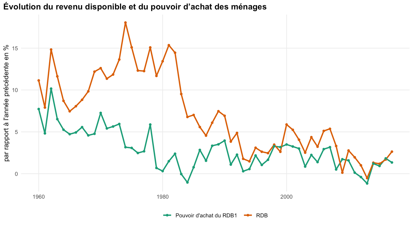

Contributions à l’évolution du pouvoir d’achat des ménages de 2012 à 2017

d4 |>
  filter(!is.na(valeur), !is.na(annee), !total100) |>
  ggplot(aes(x = annee, y = valeur, color = cle, group = cle)) +
  geom_line(linewidth = 1.1) +
  geom_point(size = 1.4) +
  scale_color_brewer(palette = "Dark2", name = NULL, labels = scales::label_wrap(45)) +
  theme_pub() +
  labs(x = NULL, y = "en points",
       title = str_wrap("Contributions à l'évolution du pouvoir d'achat des ménages de 2012 à 2017", 75)) +
  guides(color = guide_legend(ncol = 2))

Revenu disponible des ménages par habitant dans l’UE en 2016

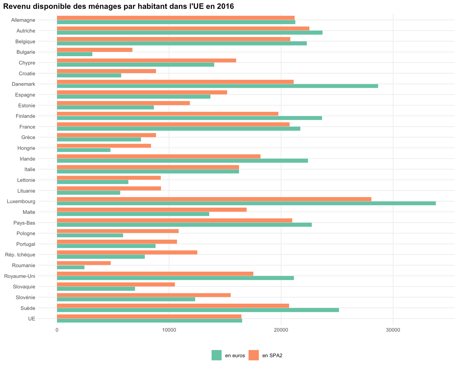
d5 |>
  filter(!is.na(valeur), !total100) |>
  mutate(lab = fct_inorder(libelle), serie = fct_inorder(serie)) |>
  ggplot(aes(x = valeur, y = fct_rev(lab), fill = serie)) +
  geom_col(position = position_dodge(width = 0.8), width = 0.75) +
  scale_y_discrete(labels = scales::label_wrap(40)) +
  scale_fill_brewer(palette = "Set2", name = NULL, labels = scales::label_wrap(30)) +
  theme_pub(10) +
  labs(x = "", y = NULL,
       title = str_wrap("Revenu disponible des ménages par habitant dans l'UE en 2016", 75)) +
  guides(fill = guide_legend(ncol = 2))