Last observation: 2025 (N = 1848)
First observation: 2020 (N = 924)
Last data update: 29 sept. 2026, 14:56
Last compile: 19 oct. 2026, 02:03
L’indicateur européen de privation matérielle et sociale mesure la part de la population dans l’incapacité de couvrir les dépenses liées à au moins cinq éléments de la vie courante sur les 13 considérés comme souhaitables, voire nécessaires, pour avoir un niveau de vie acceptable (enquête SRCV / EU-SILC).
`DS_SRCV_PMS_2025` |>
  filter(SRCV_MEASURE == "PMS", AGE == "_T", SEX == "_T", QUANTILE_NIVVIE == "_T",
         TPH == "_T", TSH == "_T", PCS == "_Z", EDUC == "_T", HLTH_SPH == "_T",
         EMPSTA_ENQ == "_T", HLTH_GALI == "_T") |>
  ggplot(aes(x = annee, y = OBS_VALUE, color = Geo)) +
  geom_line(linewidth = 1) +
  geom_point() +
  scale_color_manual(values = c("France métropolitaine" = "#1B3F8B",
                                 "France hors Mayotte" = "#E8737A"), name = NULL) +
  theme_minimal(base_size = 12) +
  labs(x = NULL, y = "%",
       title = "Taux de privation matérielle et sociale",
       subtitle = "ensemble de la population, 2020-2025") +
  theme(legend.position = "bottom", panel.grid.minor = element_blank())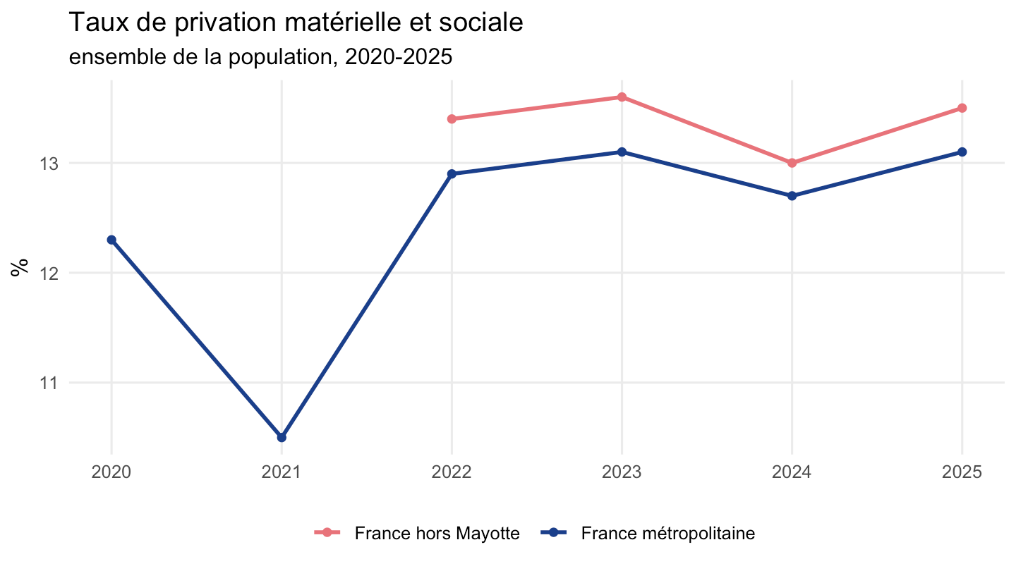
pms_by("SEX") |>
  ggplot(aes(x = annee, y = OBS_VALUE, color = Sex)) +
  geom_line(linewidth = 1) +
  geom_point() +
  scale_color_manual(values = c("Femmes" = "#E8737A", "Hommes" = "#1B3F8B"), name = NULL) +
  theme_minimal(base_size = 12) +
  labs(x = NULL, y = "%",
       title = "Taux de privation matérielle et sociale selon le sexe",
       subtitle = "France métropolitaine, 2020-2025") +
  theme(legend.position = "bottom", panel.grid.minor = element_blank())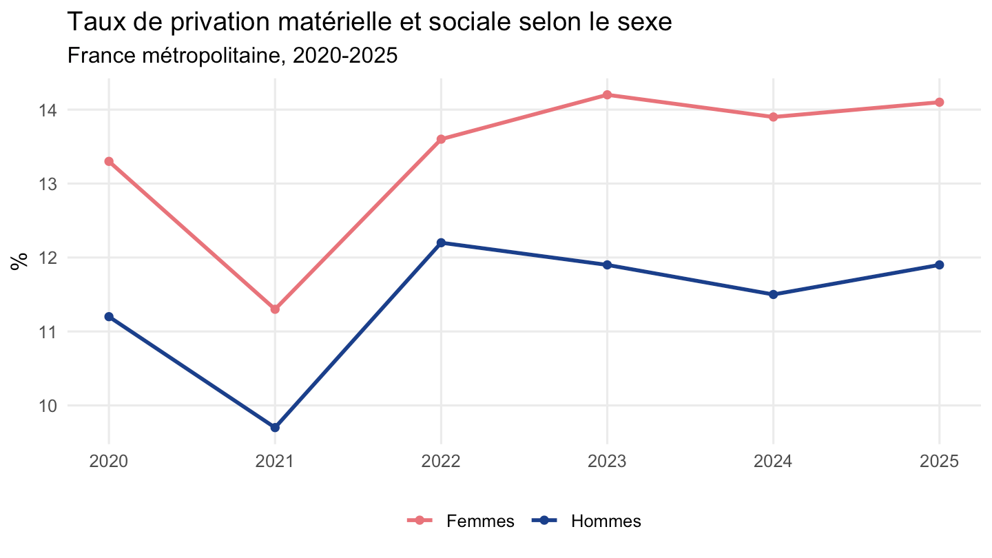
ordre_age <- c("15 ans ou moins", "De 16 à 29 ans", "De 30 à 44 ans", "De 45 à 59 ans",
                "De 60 à 74 ans", "75 ans ou plus")
pms_by("AGE") |>
  filter(annee %in% c(2020, 2025)) |>
  mutate(Age = factor(Age, levels = ordre_age)) |>
  ggplot(aes(x = Age, y = OBS_VALUE, fill = factor(annee))) +
  geom_col(position = "dodge") +
  scale_fill_manual(values = c("2020" = "#8FA8D8", "2025" = "#1B3F8B"), name = NULL) +
  theme_minimal(base_size = 10) +
  labs(x = NULL, y = "%",
       title = "Taux de privation matérielle et sociale selon l'âge",
       subtitle = "France métropolitaine, 2020 et 2025") +
  theme(legend.position = "bottom", axis.text.x = element_text(angle = 20, hjust = 1),
        panel.grid.minor = element_blank())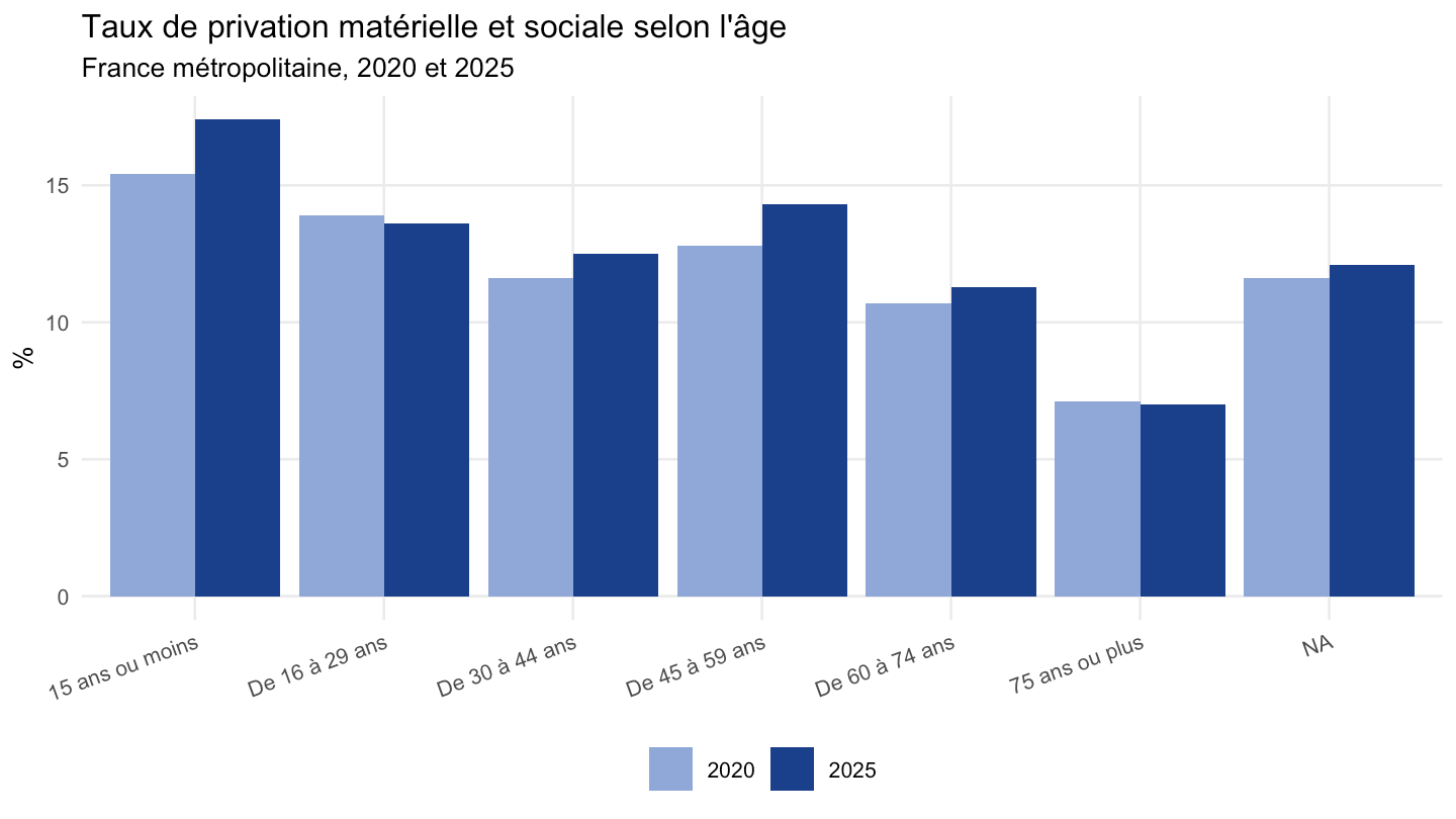
ordre_quantile <- c("Inférieur au 1er quintile", "Entre le 1er et le 2e quintile",
                     "Entre le 2e et le 3e quintile", "Entre le 3e et le 4e quintile",
                     "Supérieur au 4e quintile")
pms_by("QUANTILE_NIVVIE") |>
  mutate(Quantile_nivvie = factor(Quantile_nivvie, levels = ordre_quantile)) |>
  ggplot(aes(x = annee, y = OBS_VALUE, color = Quantile_nivvie)) +
  geom_line(linewidth = 1) +
  geom_point() +
  scale_color_brewer(palette = "RdYlBu", direction = -1, name = NULL) +
  theme_minimal(base_size = 11) +
  labs(x = NULL, y = "%",
       title = "Taux de privation matérielle et sociale selon le niveau de vie",
       subtitle = "France métropolitaine, 2020-2025") +
  theme(legend.position = "bottom", panel.grid.minor = element_blank()) +
  guides(color = guide_legend(ncol = 2))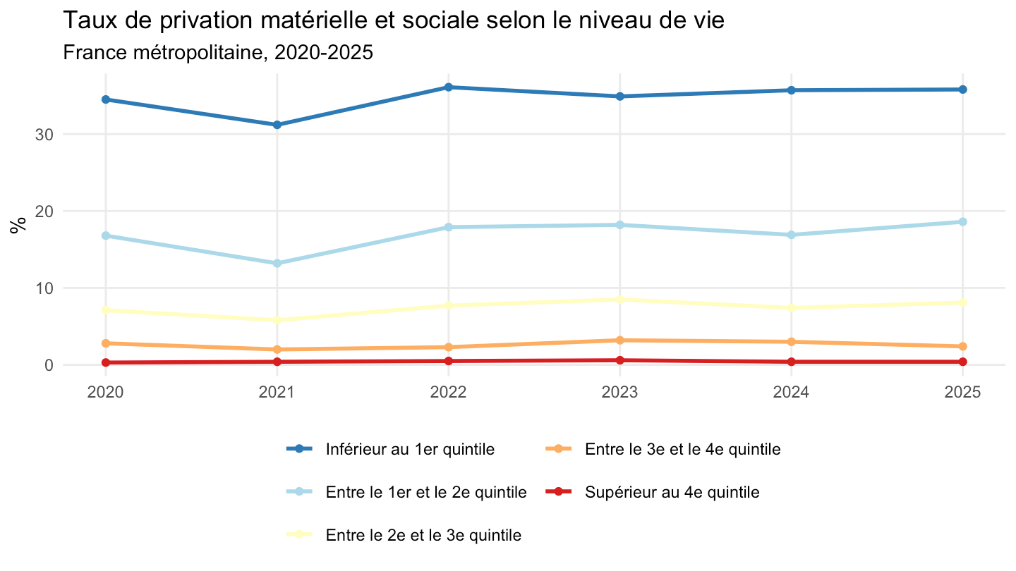
ordre_tph <- c("Personne seule", "Famille monoparentale", "Couple sans enfant résident",
               "Couple avec un enfant résident", "Couple avec deux enfants résidents",
               "Couple avec trois enfants résidents ou plus")
pms_by("TPH") |>
  filter(annee == 2025) |>
  mutate(Tph = fct_relevel(Tph, ordre_tph)) |>
  ggplot(aes(x = Tph, y = OBS_VALUE)) +
  geom_col(fill = "#1B3F8B") +
  coord_flip() +
  theme_minimal(base_size = 11) +
  labs(x = NULL, y = "%",
       title = "Taux de privation matérielle et sociale selon la composition du ménage",
       subtitle = "France métropolitaine, 2025") +
  theme(panel.grid.minor = element_blank())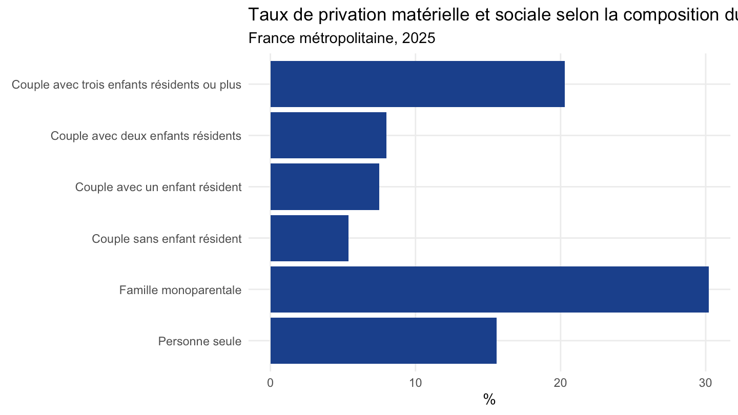
ordre_tsh <- c("Propriétaire non accédant", "Propriétaire accédant", "Locataire du parc privé",
               "Locataire du parc social")
pms_by("TSH") |>
  mutate(Tsh = factor(Tsh, levels = ordre_tsh)) |>
  ggplot(aes(x = annee, y = OBS_VALUE, color = Tsh)) +
  geom_line(linewidth = 1) +
  geom_point() +
  scale_color_manual(values = c("Propriétaire non accédant" = "#2E9E8F",
                                 "Propriétaire accédant" = "#4FA8DE",
                                 "Locataire du parc privé" = "#B08D2E",
                                 "Locataire du parc social" = "#E8737A"), name = NULL) +
  theme_minimal(base_size = 11) +
  labs(x = NULL, y = "%",
       title = "Taux de privation matérielle et sociale selon le statut d'occupation du logement",
       subtitle = "France métropolitaine, 2020-2025") +
  theme(legend.position = "bottom", panel.grid.minor = element_blank())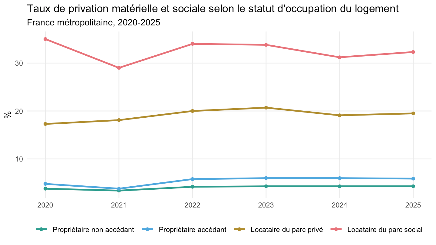
ordre_pcs <- c("Ouvriers", "Employés", "Professions intermédiaires",
               "Agriculteurs, artisans, commerçants, chefs d'entreprise",
               "Cadres et professions intellectuelles supérieures")
pms_by("PCS", age_all = FALSE) |>
  filter(annee == 2025) |>
  mutate(Pcs = factor(Pcs, levels = ordre_pcs)) |>
  ggplot(aes(x = Pcs, y = OBS_VALUE)) +
  geom_col(fill = "#1B3F8B") +
  coord_flip() +
  theme_minimal(base_size = 10) +
  labs(x = NULL, y = "%",
       title = "Taux de privation matérielle et sociale selon la catégorie socioprofessionnelle",
       subtitle = "actifs occupés de 16 ans ou plus, France métropolitaine, 2025") +
  theme(panel.grid.minor = element_blank())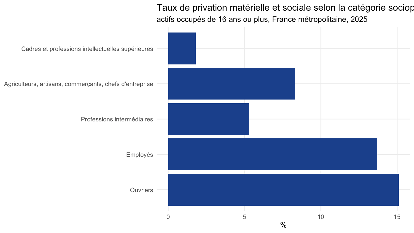
ordre_empsta <- c("Actif occupé", "Chômeur", "Retraité ou préretraité", "Autre inactif")
pms_by("EMPSTA_ENQ", age_all = FALSE) |>
  filter(annee == 2025) |>
  mutate(Empsta_enq = factor(Empsta_enq, levels = ordre_empsta)) |>
  ggplot(aes(x = Empsta_enq, y = OBS_VALUE)) +
  geom_col(fill = "#1B3F8B") +
  coord_flip() +
  theme_minimal(base_size = 11) +
  labs(x = NULL, y = "%",
       title = "Taux de privation matérielle et sociale selon la situation vis-à-vis de l'emploi",
       subtitle = "16 ans ou plus, France métropolitaine, 2025") +
  theme(panel.grid.minor = element_blank())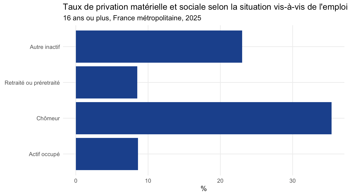
ordre_educ <- c("Aucun diplôme", "CEP, CAP, BEP, brevet des collèges ou équivalent",
                 "Baccalauréat, brevet professionnel ou équivalent",
                 "Diplôme bac+2 (Deug, DUT, BTS...)", "Diplôme supérieur à bac+2")
pms_by("EDUC", age_all = FALSE) |>
  filter(annee == 2025) |>
  mutate(Educ = factor(Educ, levels = ordre_educ)) |>
  ggplot(aes(x = Educ, y = OBS_VALUE)) +
  geom_col(fill = "#1B3F8B") +
  coord_flip() +
  theme_minimal(base_size = 9) +
  labs(x = NULL, y = "%",
       title = "Taux de privation matérielle et sociale selon le diplôme",
       subtitle = "16 ans ou plus, France métropolitaine, 2025") +
  theme(panel.grid.minor = element_blank())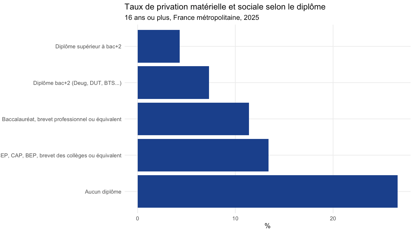
ordre_sph <- c("Très bon", "Bon", "Assez bon", "Mauvais ou très mauvais")
pms_by("HLTH_SPH", age_all = FALSE) |>
  filter(annee == 2025) |>
  mutate(Hlth_sph = factor(Hlth_sph, levels = ordre_sph)) |>
  ggplot(aes(x = Hlth_sph, y = OBS_VALUE)) +
  geom_col(fill = "#1B3F8B") +
  theme_minimal(base_size = 11) +
  labs(x = "État de santé perçu", y = "%",
       title = "Taux de privation matérielle et sociale selon l'état de santé perçu",
       subtitle = "16 ans ou plus, France métropolitaine, 2025") +
  theme(panel.grid.minor = element_blank())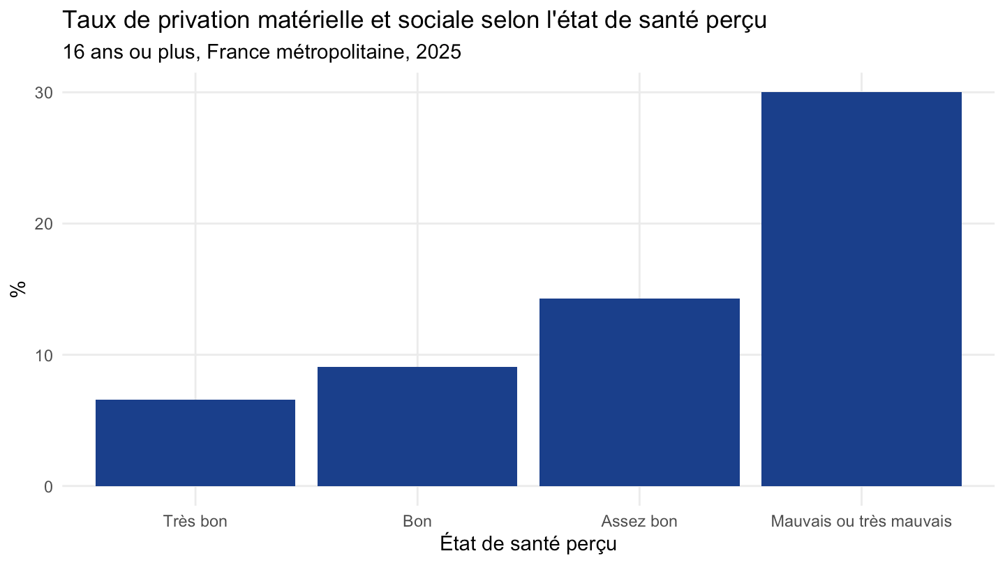
ordre_gali <- c("Pas limité du tout", "Limité mais pas fortement",
                 "Fortement limité dans ses activités courantes")
pms_by("HLTH_GALI", age_all = FALSE) |>
  filter(annee == 2025) |>
  mutate(Hlth_gali = factor(Hlth_gali, levels = ordre_gali)) |>
  ggplot(aes(x = Hlth_gali, y = OBS_VALUE)) +
  geom_col(fill = "#1B3F8B") +
  coord_flip() +
  theme_minimal(base_size = 10) +
  labs(x = NULL, y = "%",
       title = "Taux de privation matérielle et sociale selon la limitation d'activité",
       subtitle = "indicateur GALI, 16 ans ou plus, France métropolitaine, 2025") +
  theme(panel.grid.minor = element_blank())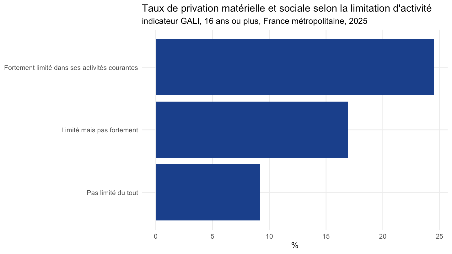
`DS_SRCV_PMS_2025` |>
  filter(GEO == "FM", annee == 2025, SRCV_MEASURE != "PMS", AGE == "_T", SEX == "_T",
         QUANTILE_NIVVIE == "_T", TPH == "_T", TSH == "_T", PCS == "_Z", EDUC == "_T",
         HLTH_SPH == "_T", EMPSTA_ENQ == "_T", HLTH_GALI == "_T") |>
  mutate(Srcv_measure = fct_reorder(Srcv_measure, OBS_VALUE)) |>
  ggplot(aes(x = Srcv_measure, y = OBS_VALUE)) +
  geom_col(fill = "#1B3F8B") +
  coord_flip() +
  theme_minimal(base_size = 9) +
  labs(x = NULL, y = "%",
       title = "Proportion de personnes déclarant subir chaque privation",
       subtitle = "France métropolitaine, 2025") +
  theme(panel.grid.minor = element_blank())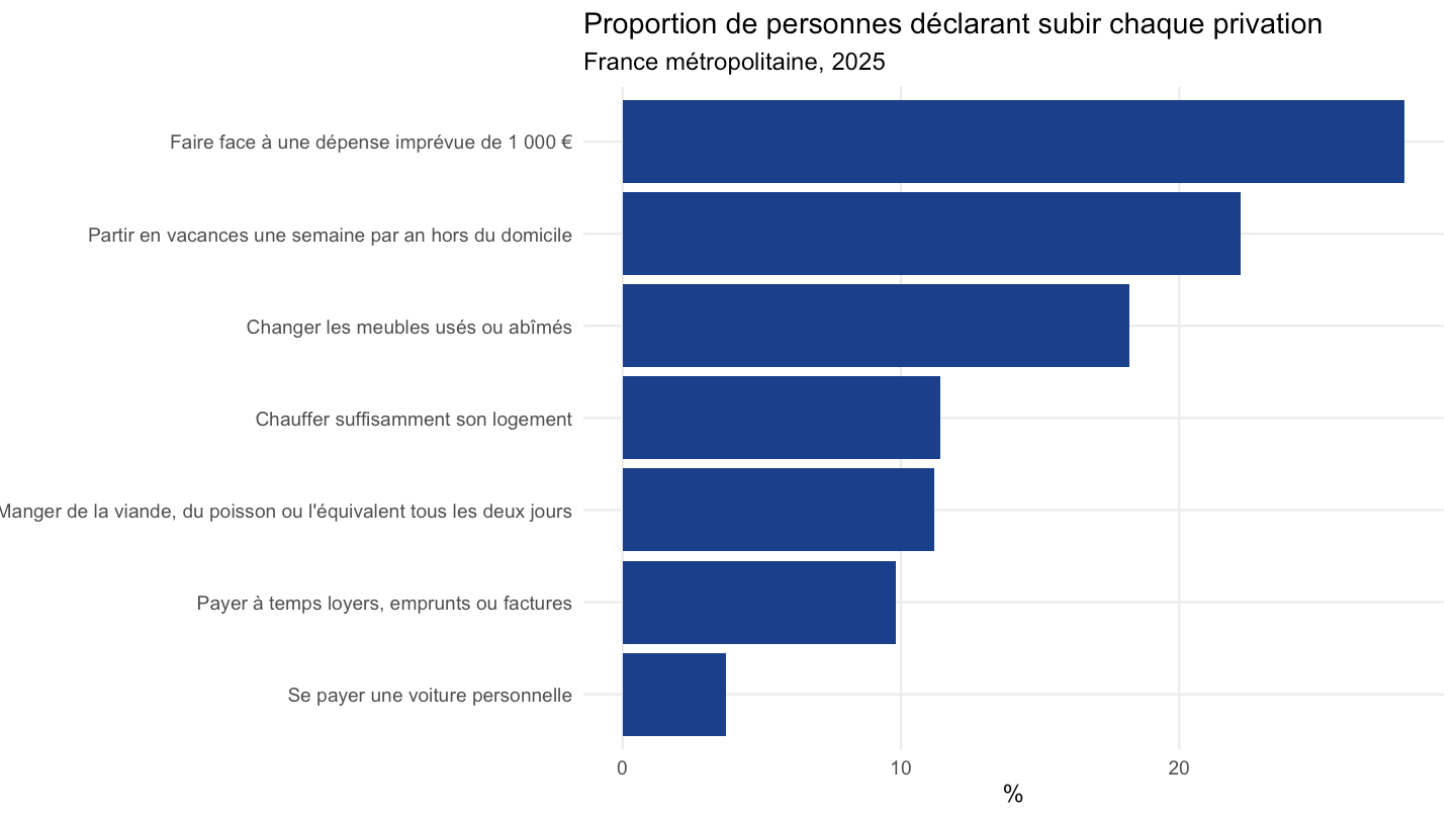
`DS_SRCV_PMS_2025` |>
  filter(GEO == "FM", SRCV_MEASURE != "PMS", AGE == "_T", SEX == "_T",
         QUANTILE_NIVVIE == "_T", TPH == "_T", TSH == "_T", PCS == "_Z", EDUC == "_T",
         HLTH_SPH == "_T", EMPSTA_ENQ == "_T", HLTH_GALI == "_T") |>
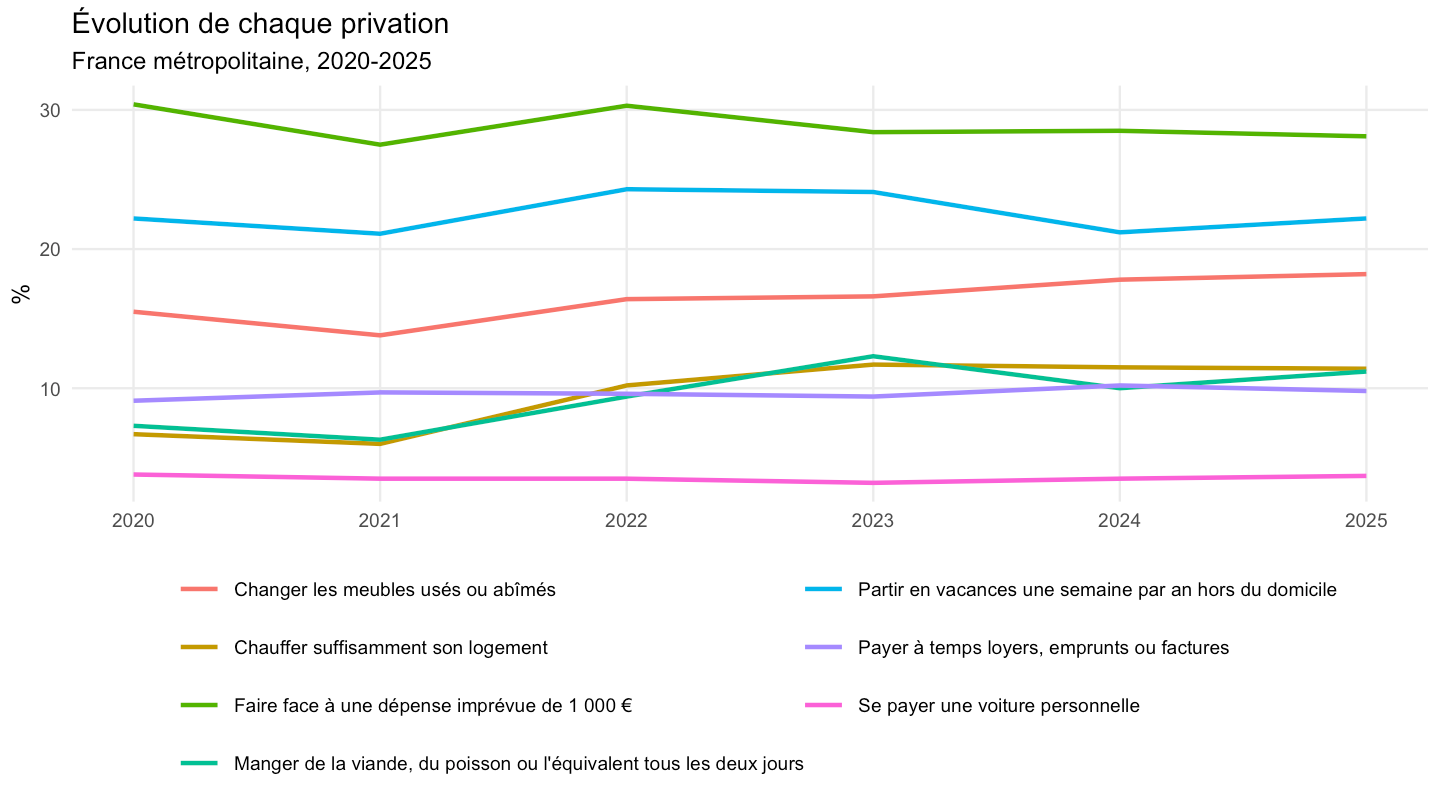
  ggplot(aes(x = annee, y = OBS_VALUE, color = Srcv_measure)) +
  geom_line(linewidth = 0.8) +
  theme_minimal(base_size = 9) +
  labs(x = NULL, y = "%",
       title = "Évolution de chaque privation",
       subtitle = "France métropolitaine, 2020-2025") +
  theme(legend.position = "bottom", panel.grid.minor = element_blank()) +
  guides(color = guide_legend(ncol = 2, title = NULL))