WEO %>%
time_to_date %>%
left_join(REF_AREA, by = "REF_AREA") %>%
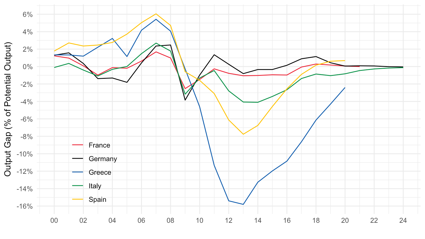
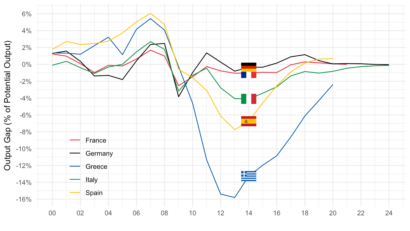
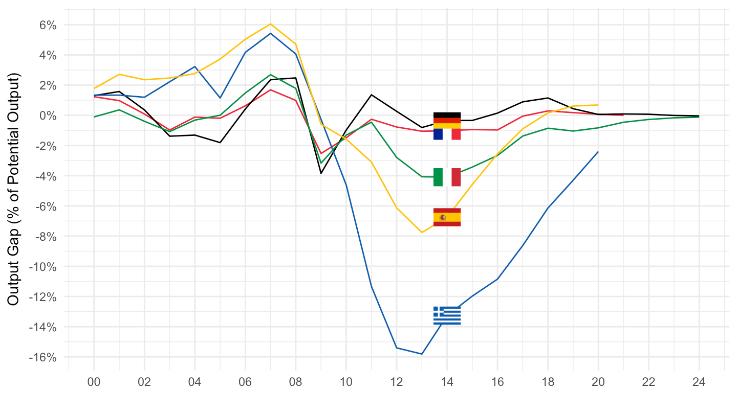
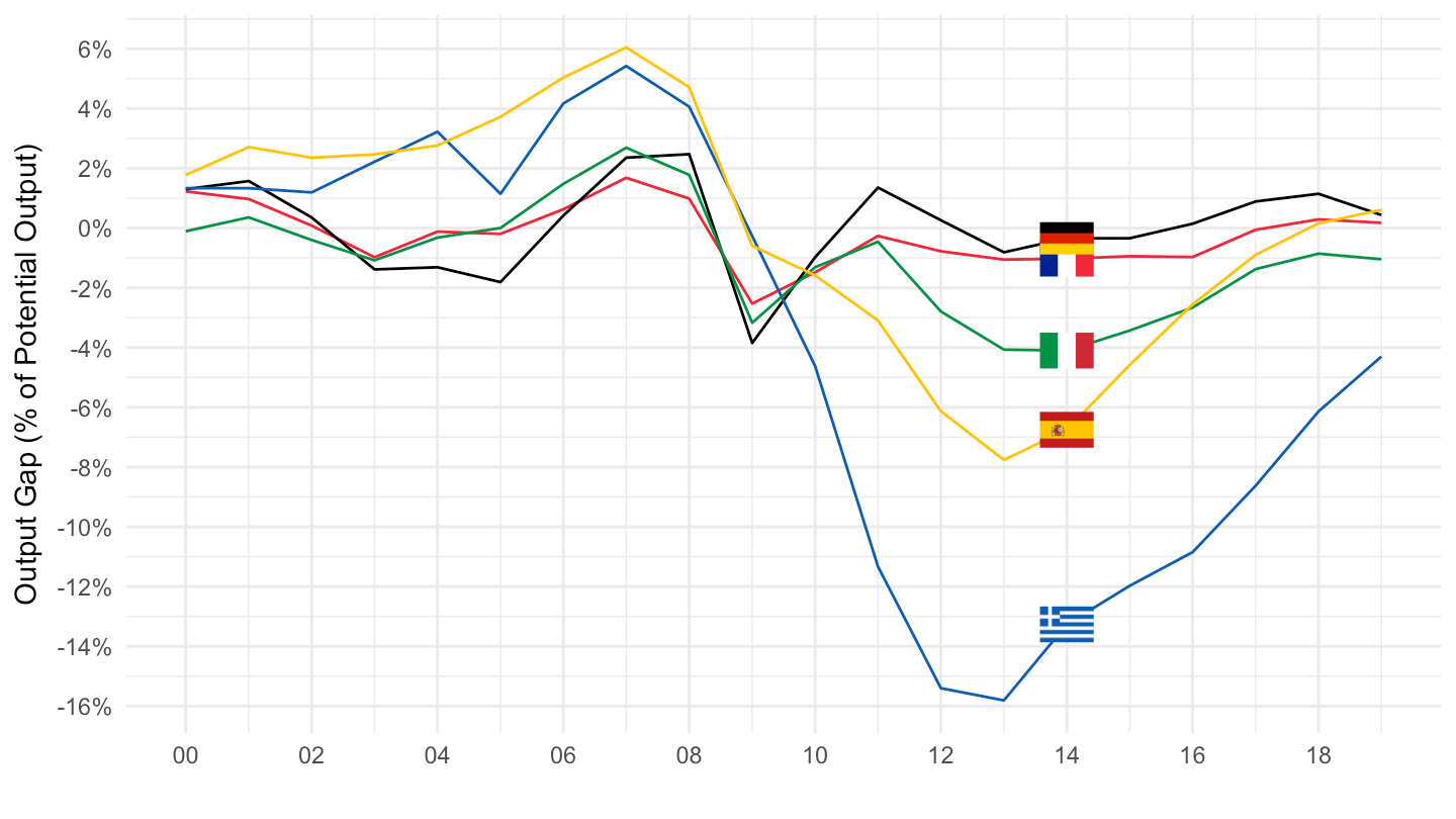
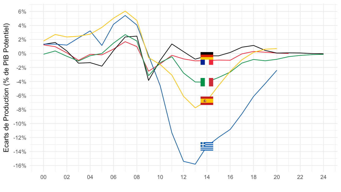
filter(CONCEPT == "NGAP_NPGDP",
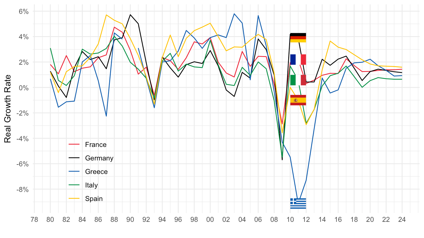
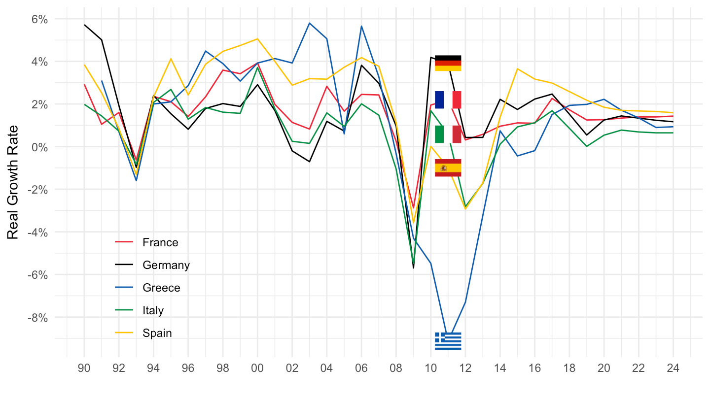
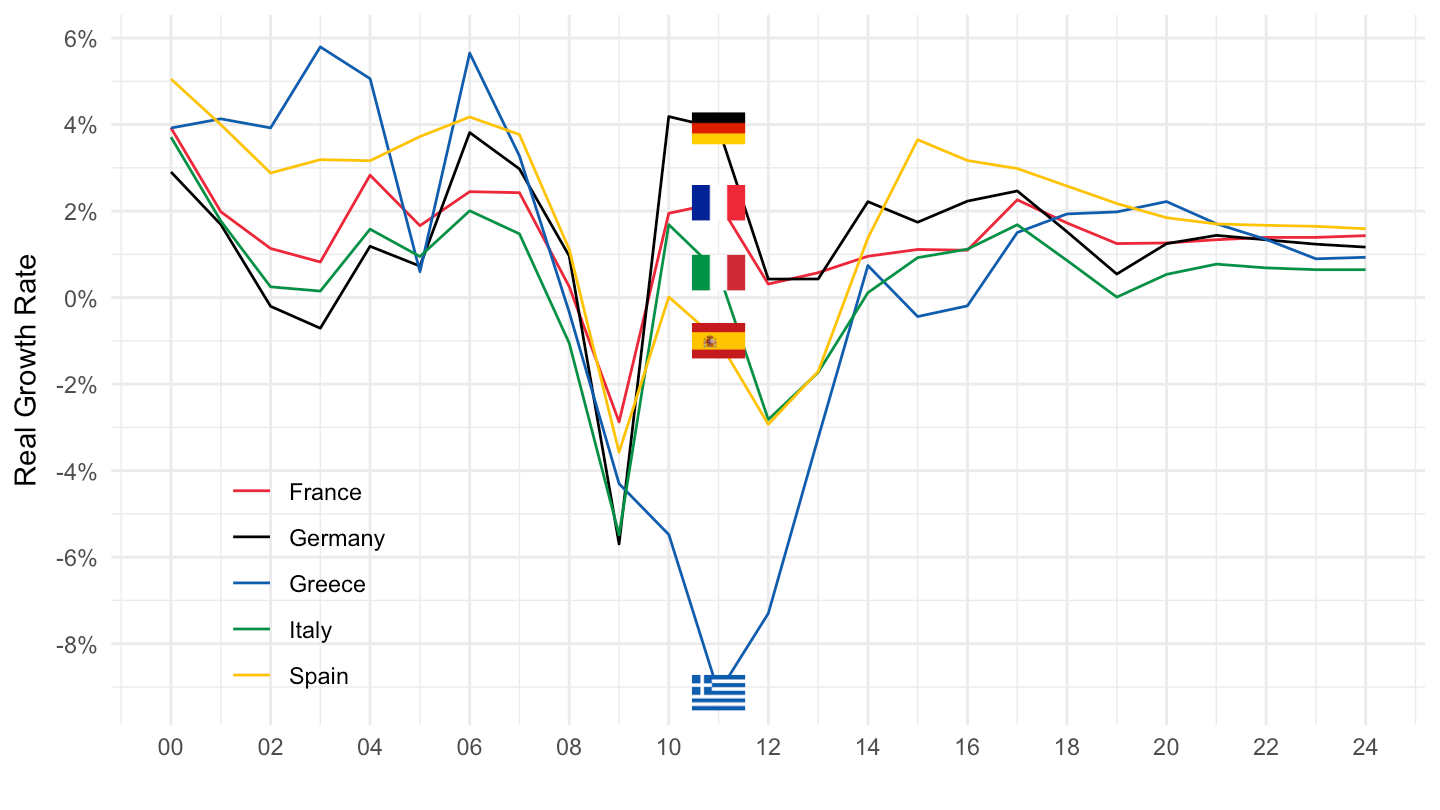
Ref_area %in% c("Italy", "France", "Greece", "Spain", "Germany"),
date >= as.Date("2000-01-01")) %>%
mutate(OBS_VALUE = OBS_VALUE/100) %>%
left_join(colors, by = c("Ref_area" = "country")) %>%
ggplot() + scale_color_identity() + add_flags +
geom_line(aes(x = date, y = OBS_VALUE, color = color)) +
theme_minimal() +
scale_x_date(breaks = seq(1920, 2100, 2) %>% paste0("-01-01") %>% as.Date,
labels = date_format("%Y")) +
theme(legend.position = c(0.15, 0.2),
legend.title = element_blank()) +
scale_y_continuous(breaks = 0.01*seq(-90, 90, 2),
labels = percent_format(accuracy = 1)) +
ylab("Output Gap (% of Potential Output)") + xlab("")