Code
WEO %>%
  left_join(CONCEPT, by = "CONCEPT") %>%
  left_join(UNIT, by = "UNIT") %>%
  group_by(CONCEPT, Concept, Unit) %>%
  summarise(Nobs = n()) %>%
  arrange(-Nobs) %>%
print_table_conditional()Data - IMF
WEO %>%
left_join(CONCEPT, by = "CONCEPT") %>%
left_join(UNIT, by = "UNIT") %>%
group_by(CONCEPT, Concept, Unit) %>%
summarise(Nobs = n()) %>%
arrange(-Nobs) %>%
print_table_conditional()WEO %>%
left_join(REF_AREA, by = "REF_AREA") %>%
group_by(REF_AREA, Ref_area) %>%
summarise(Nobs = n()) %>%
arrange(-Nobs) %>%
mutate(Flag = gsub(" ", "-", str_to_lower(gsub(" ", "-", Ref_area))),
Flag = paste0('<img src="../../icon/flag/vsmall/', Flag, '.png" alt="Flag">')) %>%
select(Flag, everything()) %>%
{if (is_html_output()) datatable(., filter = 'top', rownames = F, escape = F) else .}WEO %>%
group_by(TIME_PERIOD) %>%
summarise(Nobs = n()) %>%
arrange(desc(TIME_PERIOD)) %>%
print_table_conditional()WEO %>%
left_join(REF_AREA, by = "REF_AREA") %>%
filter(CONCEPT == "NGDPD") %>%
arrange(Ref_area, OBS_VALUE) %>%
group_by(REF_AREA, Ref_area) %>%
arrange(TIME_PERIOD) %>%
summarise(Nobs = n(),
date1 = first(TIME_PERIOD),
value1 = first(OBS_VALUE),
date2 = last(TIME_PERIOD),
value2 = last(OBS_VALUE)) %>%
mutate(Flag = gsub(" ", "-", str_to_lower(gsub(" ", "-", Ref_area))),
Flag = paste0('<img src="../../icon/flag/vsmall/', Flag, '.png" alt="Flag">')) %>%
select(Flag, everything()) %>%
{if (is_html_output()) datatable(., filter = 'top', rownames = F, escape = F) else .}WEO %>%
time_to_date %>%
left_join(REF_AREA, by = "REF_AREA") %>%
filter(CONCEPT == "NGAP_NPGDP",
Ref_area %in% c("Italy", "France", "Greece", "Spain", "Germany"),
date >= as.Date("2000-01-01")) %>%
mutate(OBS_VALUE = OBS_VALUE/100) %>%
left_join(colors, by = c("Ref_area" = "country")) %>%
ggplot() +
geom_line(aes(x = date, y = OBS_VALUE, color = color)) +
scale_color_identity() + theme_minimal() +
add_5flags +
scale_x_date(breaks = seq(1920, 2025, 2) %>% paste0("-01-01") %>% as.Date,
labels = date_format("%y")) +
scale_y_continuous(breaks = 0.01*seq(-90, 90, 2),
labels = percent_format(accuracy = 1)) +
ylab("Output Gap (% of Potential Output)") + xlab("")
WEO %>%
  time_to_date %>%
  left_join(REF_AREA, by = "REF_AREA") %>%
  filter(CONCEPT == "NGAP_NPGDP",
         Ref_area %in% c("Italy", "France", "Greece", "Spain", "Germany"),
         date >= as.Date("2000-01-01")) %>%
  mutate(OBS_VALUE = OBS_VALUE/100) %>%
  left_join(colors, by = c("Ref_area" = "country")) %>%
  ggplot() +
  geom_line(aes(x = date, y = OBS_VALUE, color = color)) +
  scale_color_identity() + theme_minimal() +
  add_5flags +
  scale_x_date(breaks = seq(1920, 2025, 2) %>% paste0("-01-01") %>% as.Date,
               labels = date_format("%y")) +
  scale_y_continuous(breaks = 0.01*seq(-90, 90, 2),
                     labels = percent_format(accuracy = 1)) +
  ylab("Output Gap (% of Potential Output)") + xlab("")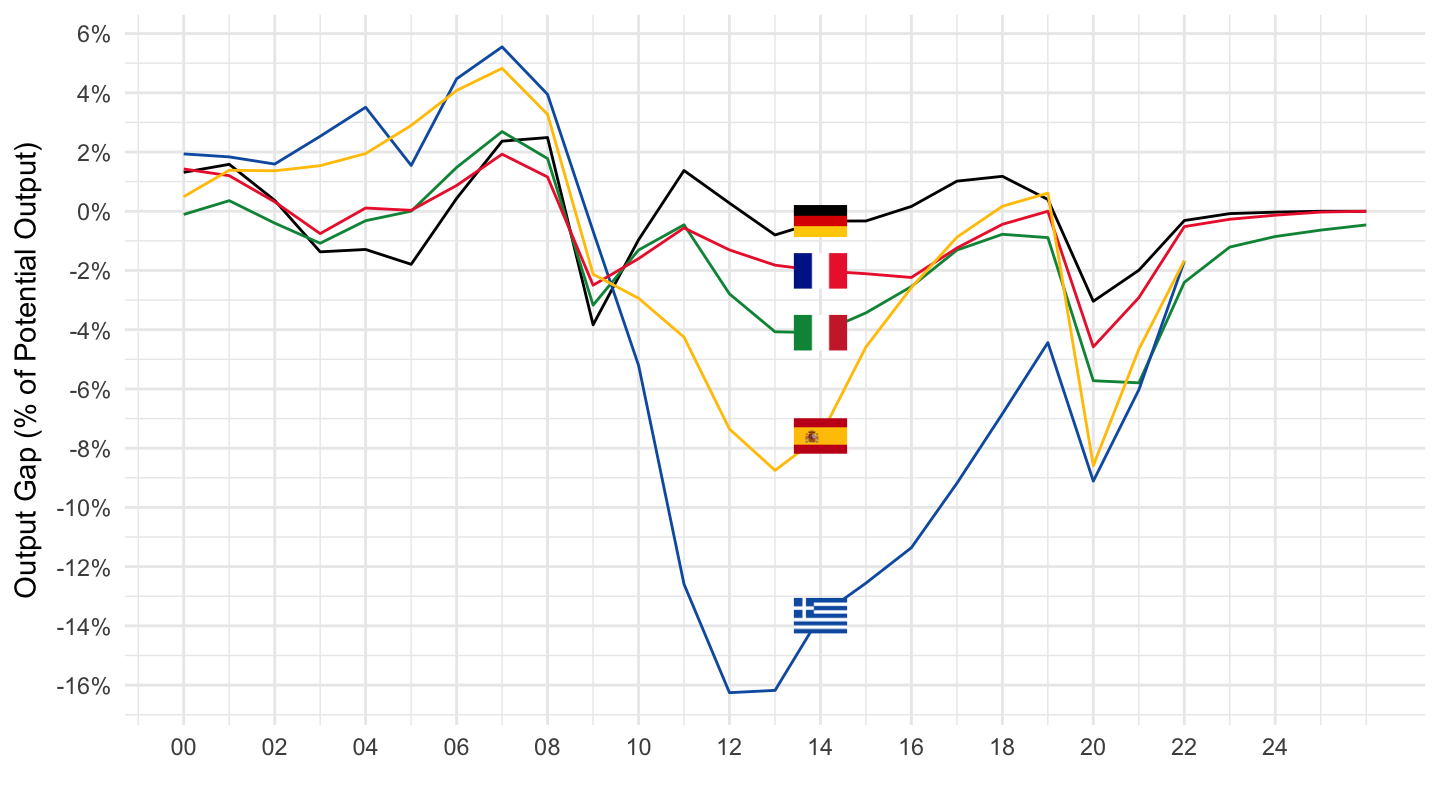
WEO %>%
time_to_date %>%
left_join(REF_AREA, by = "REF_AREA") %>%
filter(CONCEPT == "NGAP_NPGDP",
Ref_area %in% c("Italy", "France", "Greece", "Spain", "Germany"),
date >= as.Date("2000-01-01"),
date <= as.Date("2019-01-01")) %>%
mutate(OBS_VALUE = OBS_VALUE/100) %>%
left_join(colors, by = c("Ref_area" = "country")) %>%
ggplot() +
geom_line(aes(x = date, y = OBS_VALUE, color = color)) +
scale_color_identity() + theme_minimal() +
add_5flags +
scale_x_date(breaks = seq(1920, 2025, 2) %>% paste0("-01-01") %>% as.Date,
labels = date_format("%y")) +
scale_y_continuous(breaks = 0.01*seq(-90, 90, 2),
labels = percent_format(accuracy = 1)) +
ylab("Output Gap (% of Potential Output)") + xlab("")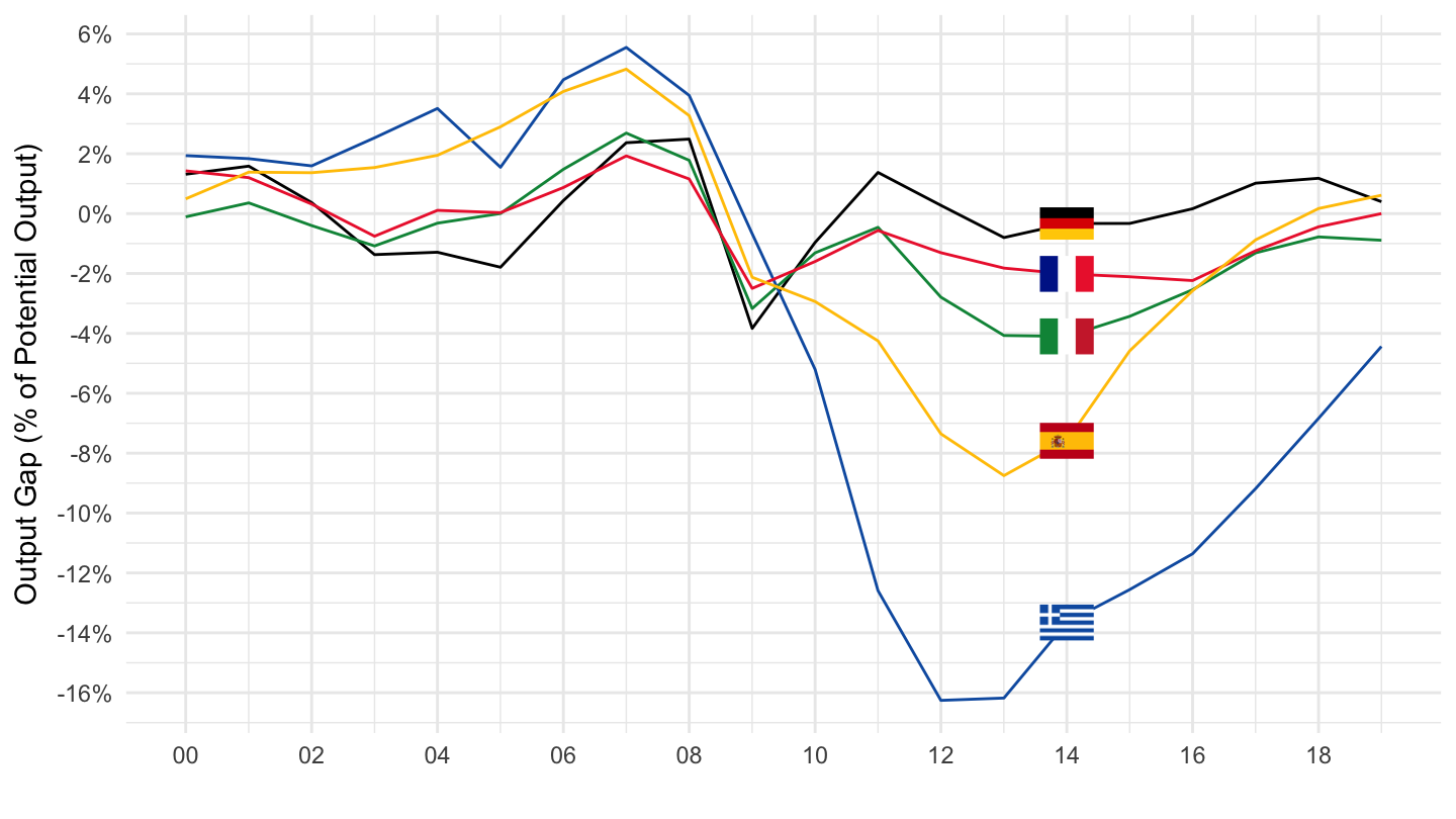
WEO %>%
  time_to_date %>%
  left_join(REF_AREA, by = "REF_AREA") %>%
  filter(CONCEPT == "NGAP_NPGDP",
         Ref_area %in% c("Italy", "France", "Greece", "Spain", "Germany"),
         date >= as.Date("2000-01-01")) %>%
  mutate(OBS_VALUE = OBS_VALUE/100) %>%
  left_join(colors, by = c("Ref_area" = "country")) %>%
  ggplot() +
  geom_line(aes(x = date, y = OBS_VALUE, color = color)) +
  scale_color_identity() + theme_minimal() +
  add_5flags +
  scale_x_date(breaks = seq(1920, 2025, 2) %>% paste0("-01-01") %>% as.Date,
               labels = date_format("%y")) +
  scale_y_continuous(breaks = 0.01*seq(-90, 90, 2),
                     labels = percent_format(accuracy = 1)) +
  ylab("Output Gap (% of Potential Output)") + xlab("")
WEO %>%
  left_join(REF_AREA, by = "REF_AREA") %>%
  time_to_date %>%
  filter(CONCEPT == "NGDP_RPCH",
         Ref_area %in% c("Italy", "France", "Greece", "Spain", "Germany")) %>%
  mutate(OBS_VALUE = OBS_VALUE/100) %>%
  left_join(colors, by = c("Ref_area" = "country")) %>%
  ggplot() + add_5flags + scale_color_identity() + theme_minimal() +
  geom_line(aes(x = date, y = OBS_VALUE, color = color)) +
  ylab("Real Growth Rate") + xlab("") +
  scale_x_date(breaks = seq(1920, 2025, 2) %>% paste0("-01-01") %>% as.Date,
               labels = date_format("%y")) +
  scale_y_continuous(breaks = 0.01*seq(-90, 90, 2),
                     labels = percent_format(accuracy = 1))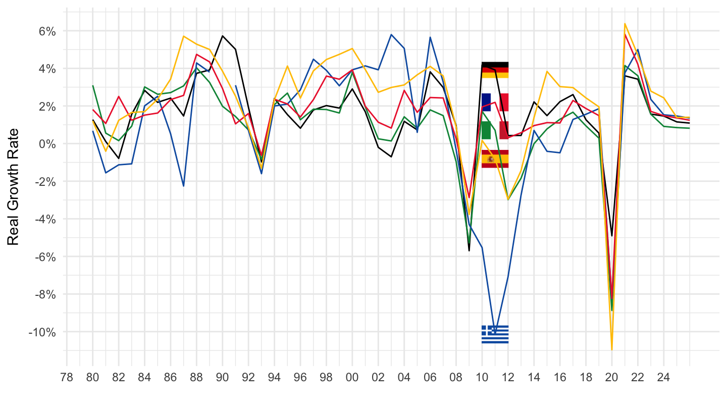
WEO %>%
  left_join(REF_AREA, by = "REF_AREA") %>%
  time_to_date %>%
  filter(CONCEPT == "NGDP_RPCH",
         Ref_area %in% c("Italy", "France", "Greece", "Spain", "Germany"),
         date >= as.Date("1990-01-01")) %>%
  mutate(OBS_VALUE = OBS_VALUE/100) %>%
  left_join(colors, by = c("Ref_area" = "country")) %>%
  ggplot() + add_5flags + scale_color_identity() + theme_minimal() +
  geom_line(aes(x = date, y = OBS_VALUE, color = color)) +
  ylab("Real Growth Rate") + xlab("") +
  scale_x_date(breaks = seq(1920, 2025, 2) %>% paste0("-01-01") %>% as.Date,
               labels = date_format("%y")) +
  scale_y_continuous(breaks = 0.01*seq(-90, 90, 2),
                     labels = percent_format(accuracy = 1))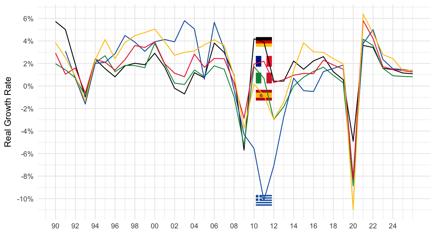
WEO %>%
  left_join(REF_AREA, by = "REF_AREA") %>%
  time_to_date %>%
  filter(CONCEPT == "NGDP_RPCH",
         Ref_area %in% c("Italy", "France", "Greece", "Spain", "Germany"),
         date >= as.Date("2000-01-01")) %>%
  mutate(OBS_VALUE = OBS_VALUE/100) %>%
  left_join(colors, by = c("Ref_area" = "country")) %>%
  ggplot() + add_5flags + scale_color_identity() + theme_minimal() +
  geom_line(aes(x = date, y = OBS_VALUE, color = color)) +
  ylab("Real Growth Rate") + xlab("") +
  scale_x_date(breaks = seq(1920, 2025, 2) %>% paste0("-01-01") %>% as.Date,
               labels = date_format("%y")) +
  scale_y_continuous(breaks = 0.01*seq(-90, 90, 2),
                     labels = percent_format(accuracy = 1))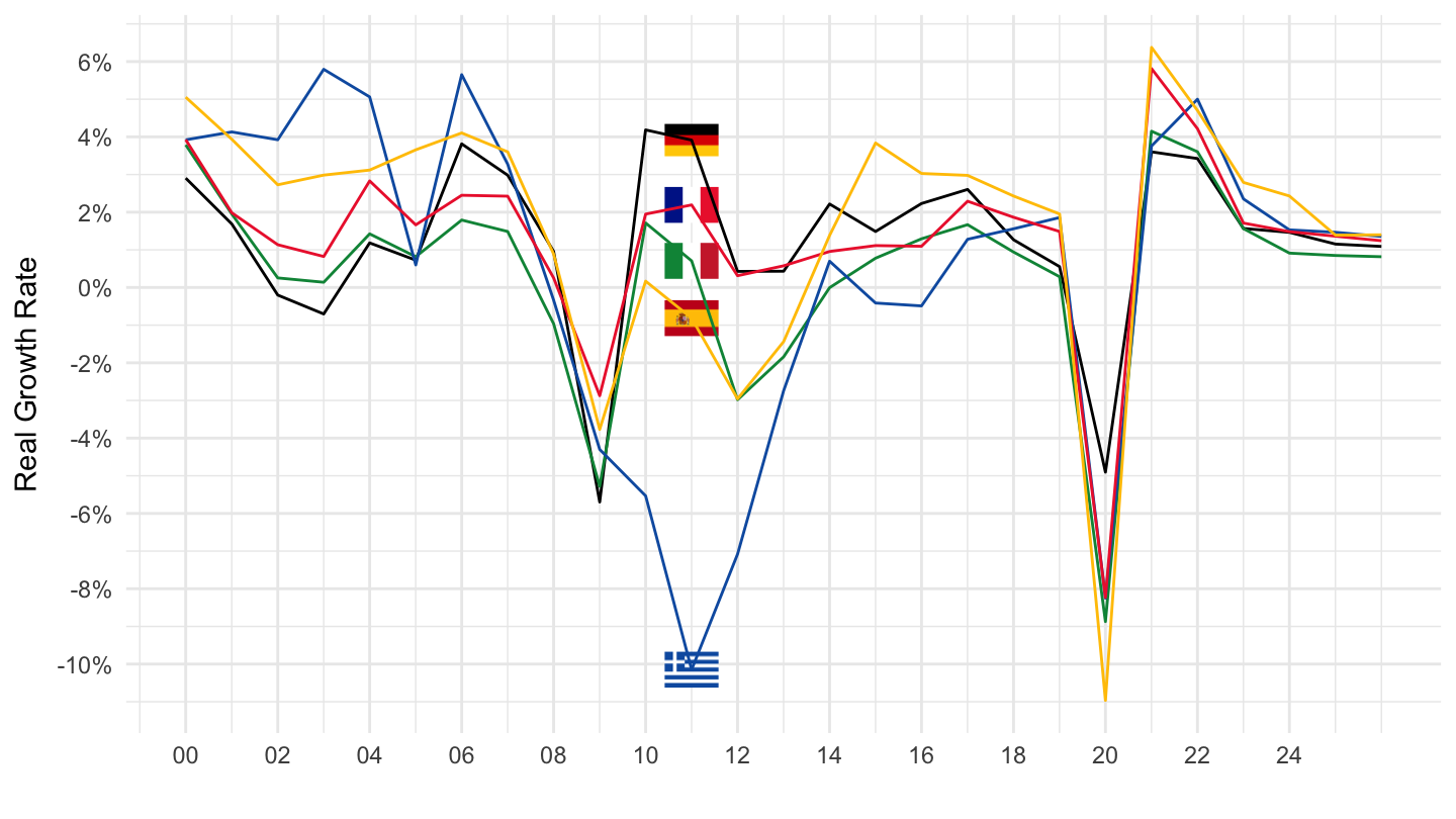
WEO %>%
  left_join(REF_AREA, by = "REF_AREA") %>%
  filter(CONCEPT == "LUR") %>%
  arrange(Ref_area, OBS_VALUE) %>%
  group_by(REF_AREA, Ref_area) %>%
  summarise(Nobs = n(),
            date1 = first(TIME_PERIOD),
            value1 = first(OBS_VALUE),
            date2 = last(TIME_PERIOD),
            value2 = last(OBS_VALUE)) %>%
  mutate(Flag = gsub(" ", "-", str_to_lower(gsub(" ", "-", Ref_area))),
         Flag = paste0('<img src="../../icon/flag/vsmall/', Flag, '.png" alt="Flag">')) %>%
  select(Flag, everything()) %>%
{if (is_html_output()) datatable(., filter = 'top', rownames = F, escape = F) else .}WEO %>%
left_join(REF_AREA, by = "REF_AREA") %>%
time_to_date %>%
filter(CONCEPT == "LUR",
Ref_area %in% c("Argentina", "Chile", "Venezuela")) %>%
mutate(OBS_VALUE = OBS_VALUE/100) %>%
left_join(colors, by = c("Ref_area" = "country")) %>%
ggplot() + add_3flags + scale_color_identity() + theme_minimal() +
geom_line(aes(x = date, y = OBS_VALUE, color = color)) +
ylab("Unemployment (%)") + xlab("") +
scale_x_date(breaks = seq(1920, 2025, 2) %>% paste0("-01-01") %>% as.Date,
labels = date_format("%y")) +
scale_y_continuous(breaks = 0.01*seq(-90, 90, 2),
labels = percent_format(accuracy = 1))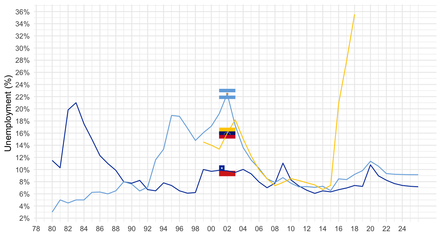
WEO %>%
  left_join(REF_AREA, by = "REF_AREA") %>%
  time_to_date %>%
  filter(CONCEPT == "LUR",
         Ref_area %in% c("France", "Italy", "Germany")) %>%
  mutate(OBS_VALUE = OBS_VALUE/100) %>%
  left_join(colors, by = c("Ref_area" = "country")) %>%
  ggplot() + add_3flags + scale_color_identity() + theme_minimal() +
  geom_line(aes(x = date, y = OBS_VALUE, color = color)) +
  ylab("Unemployment (%)") + xlab("") +
  scale_x_date(breaks = seq(1920, 2025, 2) %>% paste0("-01-01") %>% as.Date,
               labels = date_format("%y")) +
  scale_y_continuous(breaks = 0.01*seq(-90, 90, 2),
                     labels = percent_format(accuracy = 1))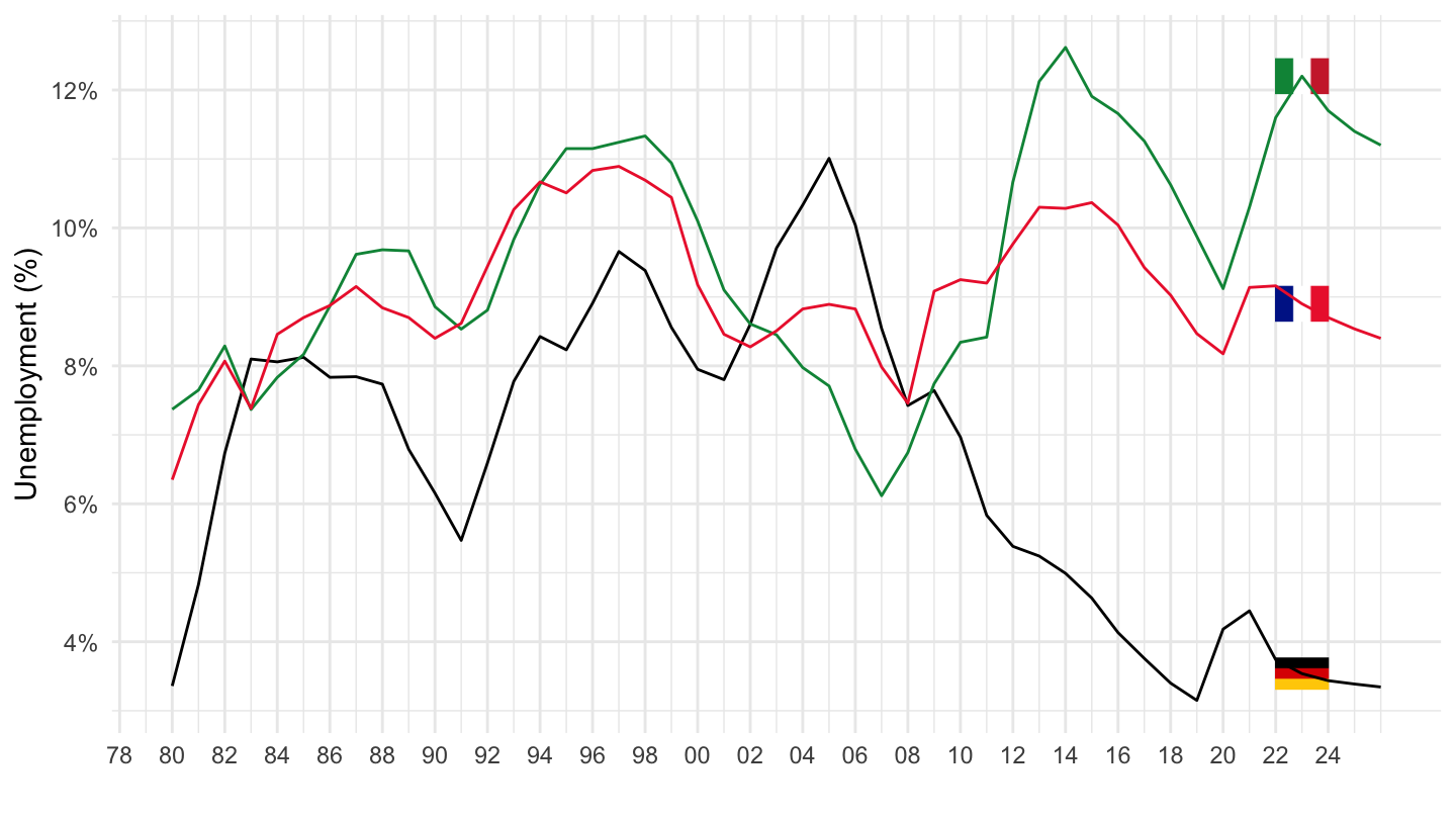
WEO %>%
  left_join(REF_AREA, by = "REF_AREA") %>%
  filter(CONCEPT == "NID_NGDP") %>%
  arrange(Ref_area, OBS_VALUE) %>%
  group_by(REF_AREA, Ref_area) %>%
  arrange(TIME_PERIOD) %>%
  summarise(Nobs = n(),
            date1 = first(TIME_PERIOD),
            value1 = first(OBS_VALUE),
            date2 = last(TIME_PERIOD),
            value2 = last(OBS_VALUE)) %>%
  mutate(Flag = gsub(" ", "-", str_to_lower(gsub(" ", "-", Ref_area))),
         Flag = paste0('<img src="../../icon/flag/vsmall/', Flag, '.png" alt="Flag">')) %>%
  select(Flag, everything()) %>%
{if (is_html_output()) datatable(., filter = 'top', rownames = F, escape = F) else .}WEO %>%
time_to_date %>%
left_join(REF_AREA, by = "REF_AREA") %>%
filter(CONCEPT == "NID_NGDP",
Ref_area %in% c("France", "Italy", "Germany")) %>%
mutate(OBS_VALUE = OBS_VALUE/100) %>%
left_join(colors, by = c("Ref_area" = "country")) %>%
ggplot() + add_3flags + scale_color_identity() + theme_minimal() +
geom_line(aes(x = date, y = OBS_VALUE, color = color)) +
ylab("Investment Rate (%)") + xlab("") +
scale_x_date(breaks = seq(1920, 2025, 2) %>% paste0("-01-01") %>% as.Date,
labels = date_format("%y")) +
scale_y_continuous(breaks = 0.01*seq(-90, 90, 2),
labels = percent_format(accuracy = 1))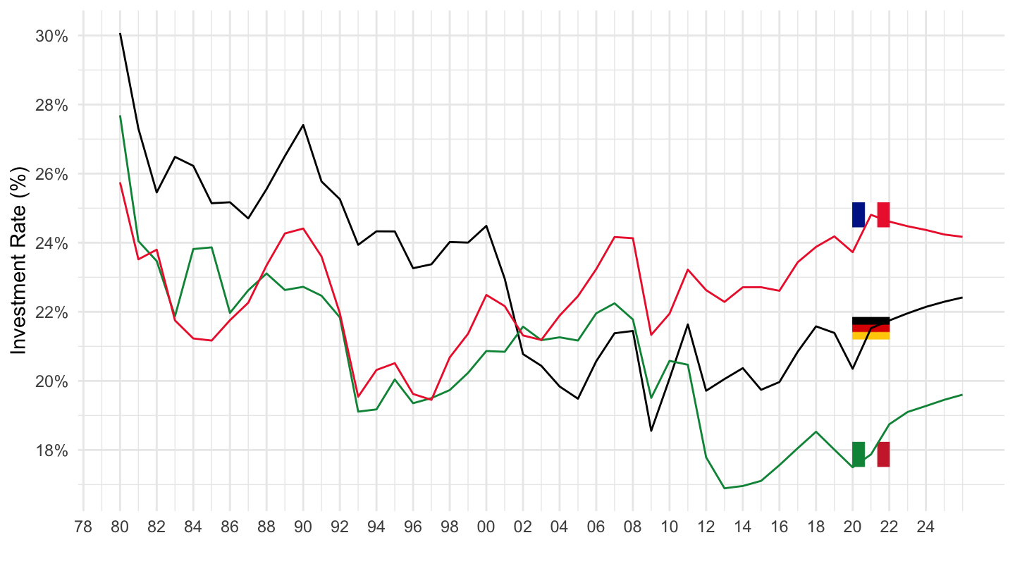
WEO %>%
  time_to_date %>%
  left_join(REF_AREA, by = "REF_AREA") %>%
  filter(CONCEPT == "NID_NGDP",
         Ref_area %in% c("Portugal", "Spain", "European Union", "Cyprus", "Greece")) %>%
  mutate(OBS_VALUE = OBS_VALUE/100) %>%
  left_join(colors, by = c("Ref_area" = "country")) %>%
  ggplot() + add_5flags + scale_color_identity() + theme_minimal() +
  geom_line(aes(x = date, y = OBS_VALUE, color = color)) +
  ylab("Investment Rate (%)") + xlab("") +
  scale_x_date(breaks = seq(1920, 2025, 2) %>% paste0("-01-01") %>% as.Date,
               labels = date_format("%y")) +
  scale_y_continuous(breaks = 0.01*seq(-90, 90, 2),
                     labels = percent_format(accuracy = 1))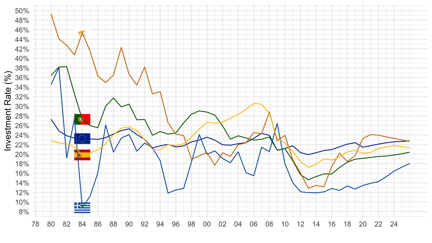
WEO %>%
  left_join(REF_AREA, by = "REF_AREA") %>%
  filter(CONCEPT == "NID_NGDP",
         Ref_area %in% c("Portugal", "Spain", "European Union", "Cyprus", "Greece")) %>%
  time_to_date %>%
  filter(date >= as.Date("1995-01-01"),
         date <= as.Date("2020-01-01")) %>%
  mutate(OBS_VALUE = OBS_VALUE/100) %>%
  left_join(colors, by = c("Ref_area" = "country")) %>%
  ggplot() + add_5flags + scale_color_identity() + theme_minimal() +
  geom_line(aes(x = date, y = OBS_VALUE, color = color)) +
  ylab("Investment Rate (%)") + xlab("") +
  scale_x_date(breaks = seq(1920, 2025, 2) %>% paste0("-01-01") %>% as.Date,
               labels = date_format("%y")) +
  scale_y_continuous(breaks = 0.01*seq(-90, 90, 2),
                     labels = percent_format(accuracy = 1))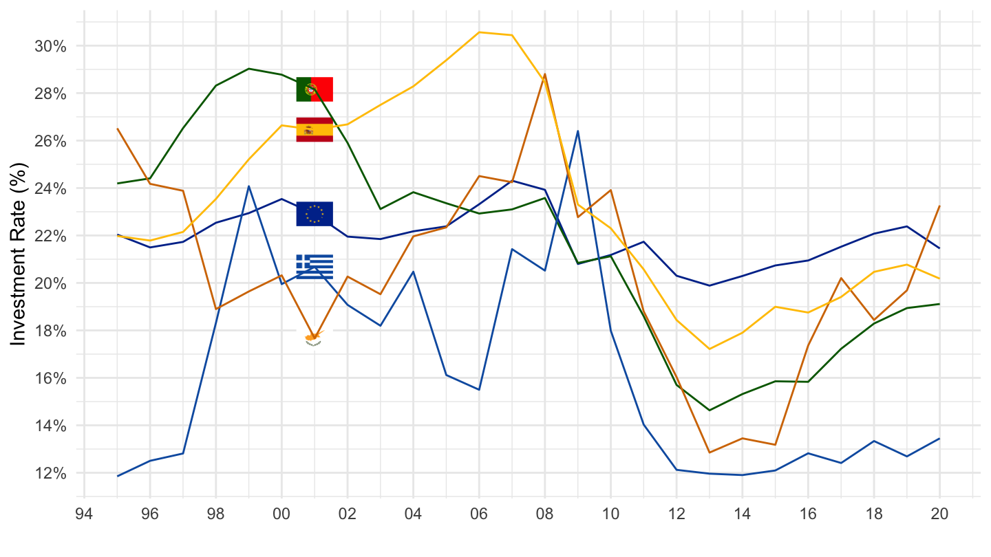
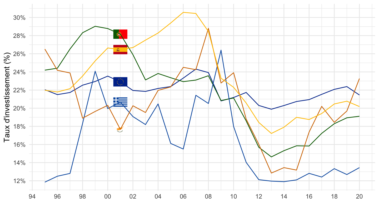
WEO %>%
  left_join(REF_AREA, by = "REF_AREA") %>%
  filter(CONCEPT == "NID_NGDP",
         Ref_area %in% c("Portugal", "Spain", "European Union", "Cyprus", "Greece")) %>%
  time_to_date %>%
  filter(date >= as.Date("1995-01-01"),
         date <= as.Date("2020-01-01")) %>%
  mutate(OBS_VALUE = OBS_VALUE/100) %>%
  left_join(colors, by = c("Ref_area" = "country")) %>%
  ggplot() + add_5flags + scale_color_identity() + theme_minimal() +
  geom_line(aes(x = date, y = OBS_VALUE, color = color)) +
  ylab("Taux d'investissement (%)") + xlab("") +
  scale_x_date(breaks = seq(1920, 2025, 2) %>% paste0("-01-01") %>% as.Date,
               labels = date_format("%y")) +
  scale_y_continuous(breaks = 0.01*seq(-90, 90, 2),
                     labels = percent_format(accuracy = 1))