Public Debt Database - MauroRomeuBinderZaman2013

Data - IMF

Author

Source: Paolo Mauro, Rafael Romeu, Ariel Binder and Asad Zaman, 2013, “A Modern History of Fiscal Prudence and Profligacy,” IMF Working Paper No. 13/5, International Monetary Fund, Washington, DC.

Variables

Code

MauroRomeuBinderZaman2013 |>
  left_join(MauroRomeuBinderZaman2013_var, by = "variable") |>
  group_by(variable, variable_desc) |>
  summarise(Nobs = n()) |>
  arrange(-Nobs) %>%
  {if (is_html_output()) datatable(., filter = 'top', rownames = F) else .}

iso2c

Code

MauroRomeuBinderZaman2013 |>
  left_join(CL_AREA_FM |> rename(iso2c = AREA), by = "iso2c") |>
  group_by(iso2c, AREA_desc) |>
  summarise(Nobs = n()) |>
  arrange(-Nobs) %>%
  {if (is_html_output()) datatable(., filter = 'top', rownames = F) else .}

Model

\[B_{t+1} = (1+i_t) B_t + D_t\]

Ex 1: Net Government Debt (% of GDP)

Code

MauroRomeuBinderZaman2013 |>
  filter(variable == "pb",
         date == as.Date("2010-01-01")) |>
  left_join(CL_AREA_FM |> rename(iso2c = AREA), by = "iso2c") |>
  select(iso2c, AREA_desc, value) |>
  arrange(-value) |>
  na.omit() %>%
  mutate_at(vars(3), funs(paste0(round(as.numeric(.), 1), " %"))) %>%
  {if (is_html_output()) datatable(., filter = 'top', rownames = F) else .}

Ex 2: Primary balance (% of GDP)

Italy, France, Germany, United States

Code

MauroRomeuBinderZaman2013 |>
  filter(variable == "pb",
         iso2c %in% c("IT", "FR", "DE", "US"),
         date >= as.Date("1945-01-01")) |>
  left_join(CL_AREA_FM |> rename(iso2c = AREA), by = "iso2c") |>
    mutate(value = value/100) |>
  left_join(colors, by = c("AREA_desc" = "country")) |>
ggplot() + scale_color_identity() + add_flags + 
  geom_line(aes(x = date, y = value, color = color)) +
  theme_minimal() +
  scale_x_date(breaks = seq(1920, 2100, 5) |> paste0("-01-01") |> as.Date(),
               labels = date_format("%Y")) +
  theme(legend.position = c(0.6, 0.3),
        legend.title = element_blank(),
        legend.direction = "horizontal") +
  scale_y_continuous(breaks = 0.01*seq(-60, 60, 2),
                     labels = scales::percent_format(accuracy = 1)) +
  ylab("Primary balance (% of GDP)") + xlab("") + 
  geom_hline(yintercept = 0, linetype = "dashed", size = 0.3)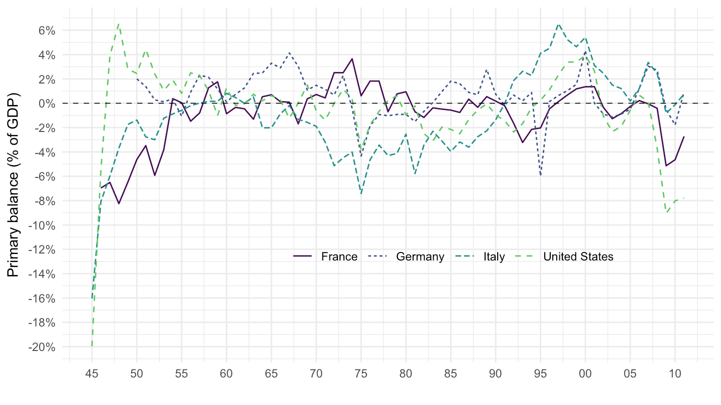

Germany, Austria, Finland, Netherlands

Code

MauroRomeuBinderZaman2013 |>
  filter(variable == "pb",
         iso2c %in% c("DE", "NL", "FI", "AT"),
         date >= as.Date("1945-01-01")) |>
  left_join(CL_AREA_FM |> rename(iso2c = AREA), by = "iso2c") |>
    mutate(value = value/100) |>
  left_join(colors, by = c("AREA_desc" = "country")) |>
ggplot() + scale_color_identity() + add_flags + 
  geom_line(aes(x = date, y = value, color = color)) +
  theme_minimal() +
  scale_x_date(breaks = seq(1920, 2100, 5) |> paste0("-01-01") |> as.Date(),
               labels = date_format("%Y")) +
  theme(legend.position = c(0.6, 0.1),
        legend.title = element_blank(),
        legend.direction = "horizontal") +
  scale_y_continuous(breaks = 0.01*seq(-60, 60, 2),
                     labels = scales::percent_format(accuracy = 1)) +
  ylab("Primary balance (% of GDP)") + xlab("") + 
  geom_hline(yintercept = 0, linetype = "dashed", size = 0.3)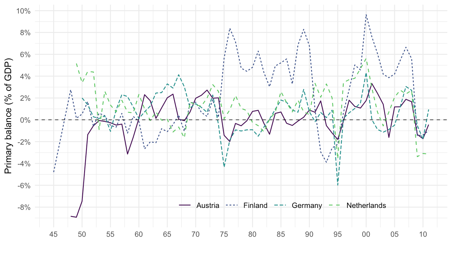

Ex 3: Interest Expense (% of GDP)

Code

MauroRomeuBinderZaman2013 |>
  filter(variable == "ie",
         iso2c %in% c("IT", "FR", "DE", "US"),
         date >= as.Date("1945-01-01")) |>
  left_join(CL_AREA_FM |> rename(iso2c = AREA), by = "iso2c") |>
    mutate(value = value/100) |>
  left_join(colors, by = c("AREA_desc" = "country")) |>
ggplot() + scale_color_identity() + add_flags + 
  geom_line(aes(x = date, y = value, color = color)) +
  theme_minimal() +
  scale_x_date(breaks = seq(1920, 2100, 5) |> paste0("-01-01") |> as.Date(),
               labels = date_format("%Y")) +
  theme(legend.position = c(0.3, 0.8),
        legend.title = element_blank()) +
  scale_y_continuous(breaks = 0.01*seq(-60, 60, 2),
                     labels = scales::percent_format(accuracy = 1)) +
  ylab("Interest Expense (% of GDP)") + xlab("")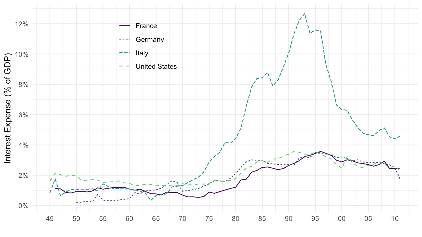

Ex 4: Debt (% of GDP)

Code

MauroRomeuBinderZaman2013 |>
  filter(variable == "d",
         iso2c %in% c("IT", "FR", "DE", "US"),
         date >= as.Date("1920-01-01")) |>
  left_join(CL_AREA_FM |> rename(iso2c = AREA), by = "iso2c") |>
    mutate(value = value/100) |>
  left_join(colors, by = c("AREA_desc" = "country")) |>
ggplot() + scale_color_identity() + add_flags + 
  geom_line(aes(x = date, y = value, color = color)) +
  theme_minimal() +
  scale_x_date(breaks = seq(1920, 2100, 5) |> paste0("-01-01") |> as.Date(),
               labels = date_format("%Y")) +
  theme(legend.position = c(0.7, 0.8),
        legend.title = element_blank()) +
  scale_y_continuous(breaks = 0.01*seq(-60, 300, 10),
                     labels = scales::percent_format(accuracy = 1)) +
  ylab("Gross Government Debt (% of GDP)") + xlab("")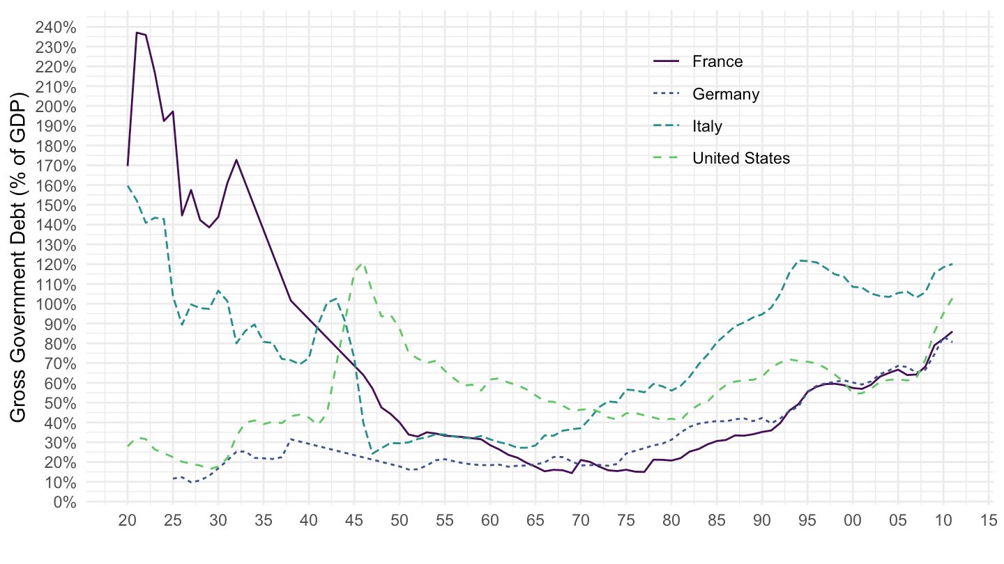

Ex 5: Debt

France

Code

MauroRomeuBinderZaman2013 |>
  filter(iso2c == "FR",
         variable %in% c("d", "ie", "pb")) |>
  select(date, variable, value) |>
  spread(variable, value) |>
  setNames(c("Date", "Debt/GDP", "Interest/GDP", "Primary Deficit/GDP")) %>%
  mutate_at(vars(2, 3, 4), funs(paste0(round(as.numeric(.), 2), " %"))) %>%
  {if (is_html_output()) datatable(., filter = 'top', rownames = F) else .}

Germany

Code

MauroRomeuBinderZaman2013 |>
  filter(iso2c == "DE",
         variable %in% c("d", "ie", "pb")) |>
  select(date, variable, value) |>
  spread(variable, value) |>
  setNames(c("Date", "Debt/GDP", "Interest/GDP", "Primary Deficit/GDP")) %>%
  mutate_at(vars(2, 3, 4), funs(paste0(round(as.numeric(.), 2), " %"))) %>%
  {if (is_html_output()) datatable(., filter = 'top', rownames = F) else .}

Ex 6: r - g

France

Code

MauroRomeuBinderZaman2013 |>
  filter(iso2c == "FR",
         # rgc: Real GDP growth rate, percent
         # rltirc: Real long term interest rate on gov't debt, percent
         variable %in% c("rgc", "rltirc"),
         date >= as.Date("1955-01-01")) |>
  left_join(MauroRomeuBinderZaman2013_var, by = "variable") |>
  ggplot() + 
  geom_line(aes(x = date, y = value/100, color = variable_desc, linetype = variable_desc)) +
  scale_color_manual(values = viridis(5)[1:4]) +
  theme_minimal() +
  scale_x_date(breaks = seq(1920, 2100, 5) |> paste0("-01-01") |> as.Date(),
               labels = date_format("%Y")) +
  theme(legend.position = c(0.6, 0.15),
        legend.title = element_blank()) +
  scale_y_continuous(breaks = 0.01*seq(-60, 60, 1),
                     labels = scales::percent_format(accuracy = 1)) +
  ylab("r, g (%)") + xlab("") + 
  geom_hline(yintercept = 0, linetype = "dashed", size = 0.3)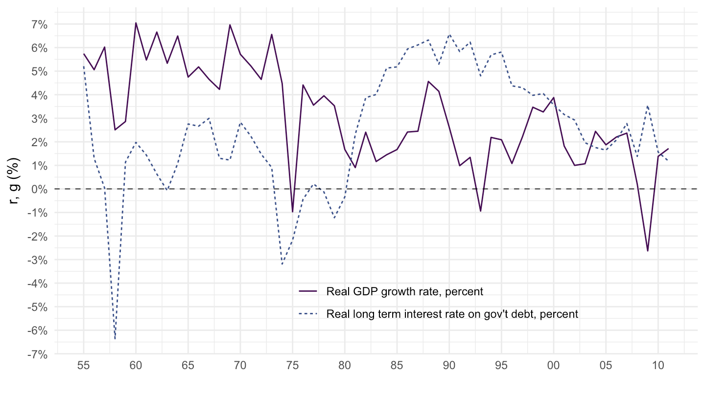

France (smoothed)

Code

MauroRomeuBinderZaman2013 |>
  filter(iso2c == "FR",
         # rgc: Real GDP growth rate, percent
         # rltirc: Real long term interest rate on gov't debt, percent
         variable %in% c("rgc", "rltirc"),
         date >= as.Date("1955-01-01")) |>
  group_by(variable) |>
  mutate(value = forecast::ma(value, 5)) |>
  left_join(MauroRomeuBinderZaman2013_var, by = "variable") |>
  ggplot() + 
  geom_line(aes(x = date, y = value/100, color = variable_desc, linetype = variable_desc)) +
  scale_color_manual(values = viridis(5)[1:4]) +
  theme_minimal() +
  scale_x_date(breaks = seq(1920, 2100, 5) |> paste0("-01-01") |> as.Date(),
               labels = date_format("%Y")) +
  theme(legend.position = c(0.6, 0.15),
        legend.title = element_blank()) +
  scale_y_continuous(breaks = 0.01*seq(-60, 60, 1),
                     labels = scales::percent_format(accuracy = 1)) +
  ylab("r, g (%)") + xlab("") + 
  geom_hline(yintercept = 0, linetype = "dashed", size = 0.3)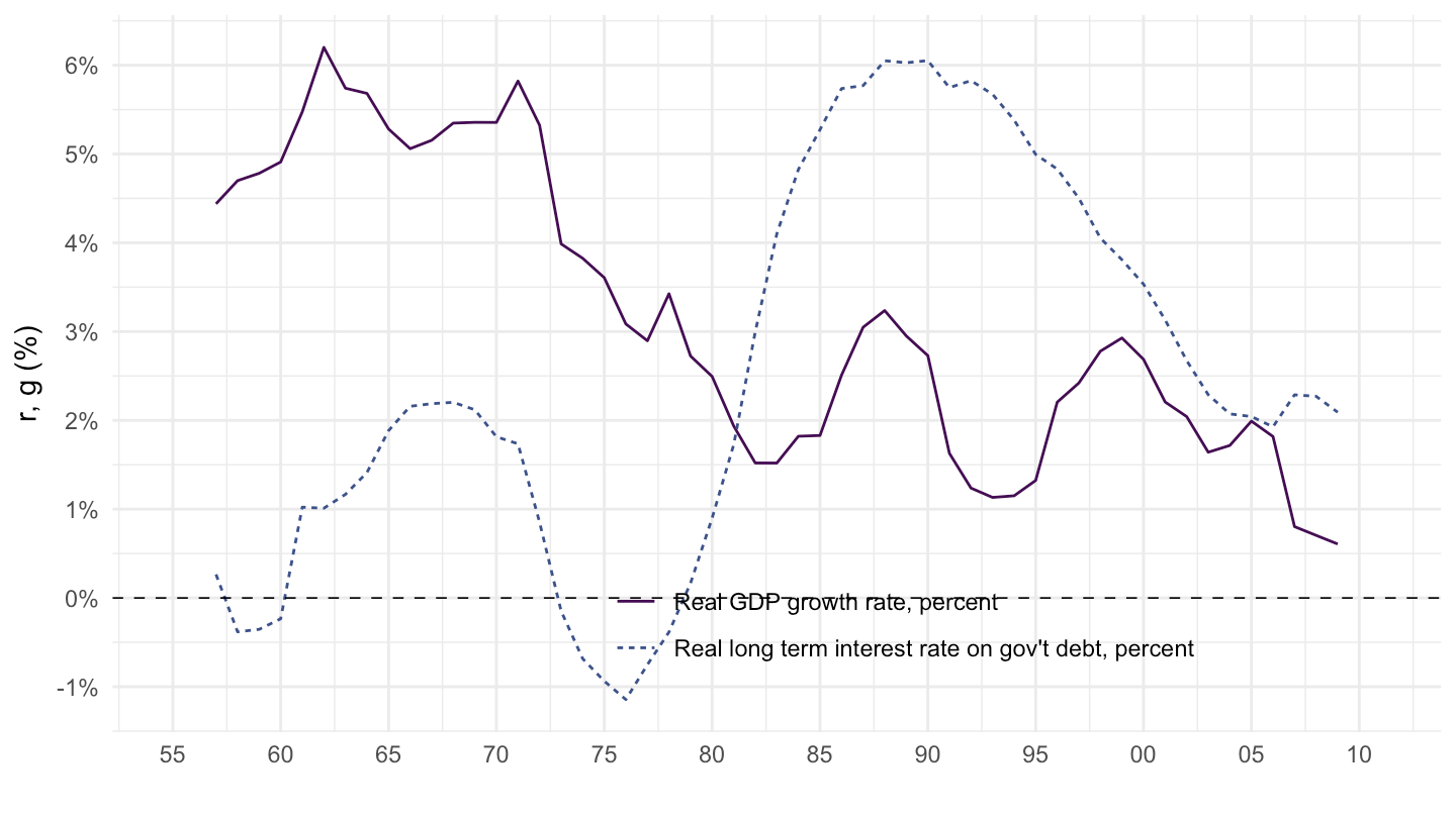

Germany

Code

MauroRomeuBinderZaman2013 |>
  filter(iso2c == "DE",
         # rgc: Real GDP growth rate, percent
         # rltirc: Real long term interest rate on gov't debt, percent
         variable %in% c("rgc", "rltirc"),
         date >= as.Date("1955-01-01")) |>
  left_join(MauroRomeuBinderZaman2013_var, by = "variable") |>
  ggplot() + 
  geom_line(aes(x = date, y = value/100, color = variable_desc, linetype = variable_desc)) +
  scale_color_manual(values = viridis(5)[1:4]) +
  theme_minimal() +
  scale_x_date(breaks = seq(1920, 2100, 5) |> paste0("-01-01") |> as.Date(),
               labels = date_format("%Y")) +
  theme(legend.position = c(0.6, 0.15),
        legend.title = element_blank()) +
  scale_y_continuous(breaks = 0.01*seq(-60, 60, 2),
                     labels = scales::percent_format(accuracy = 1)) +
  ylab("r, g (%)") + xlab("") + 
  geom_hline(yintercept = 0, linetype = "dashed", size = 0.3)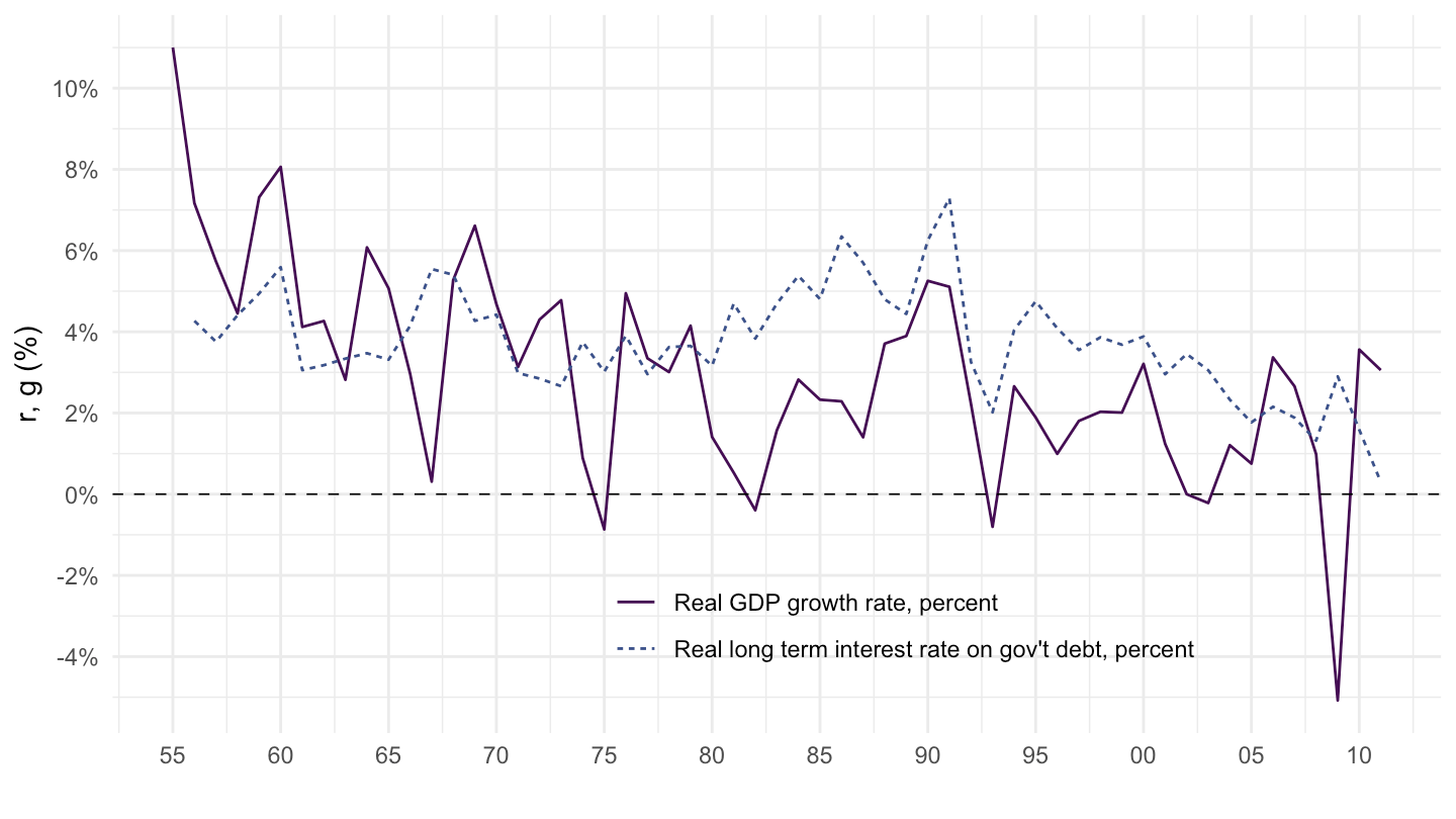

United States

Code

MauroRomeuBinderZaman2013 |>
  filter(iso2c == "US",
         # rgc: Real GDP growth rate, percent
         # rltirc: Real long term interest rate on gov't debt, percent
         variable %in% c("rgc", "rltirc"),
         date >= as.Date("1955-01-01")) |>
  left_join(MauroRomeuBinderZaman2013_var, by = "variable") |>
  ggplot() + 
  geom_line(aes(x = date, y = value/100, color = variable_desc, linetype = variable_desc)) +
  scale_color_manual(values = viridis(5)[1:4]) +
  theme_minimal() +
  scale_x_date(breaks = seq(1920, 2100, 5) |> paste0("-01-01") |> as.Date(),
               labels = date_format("%Y")) +
  theme(legend.position = c(0.6, 0.15),
        legend.title = element_blank()) +
  scale_y_continuous(breaks = 0.01*seq(-60, 60, 2),
                     labels = scales::percent_format(accuracy = 1)) +
  ylab("r, g (%)") + xlab("") + 
  geom_hline(yintercept = 0, linetype = "dashed", size = 0.3)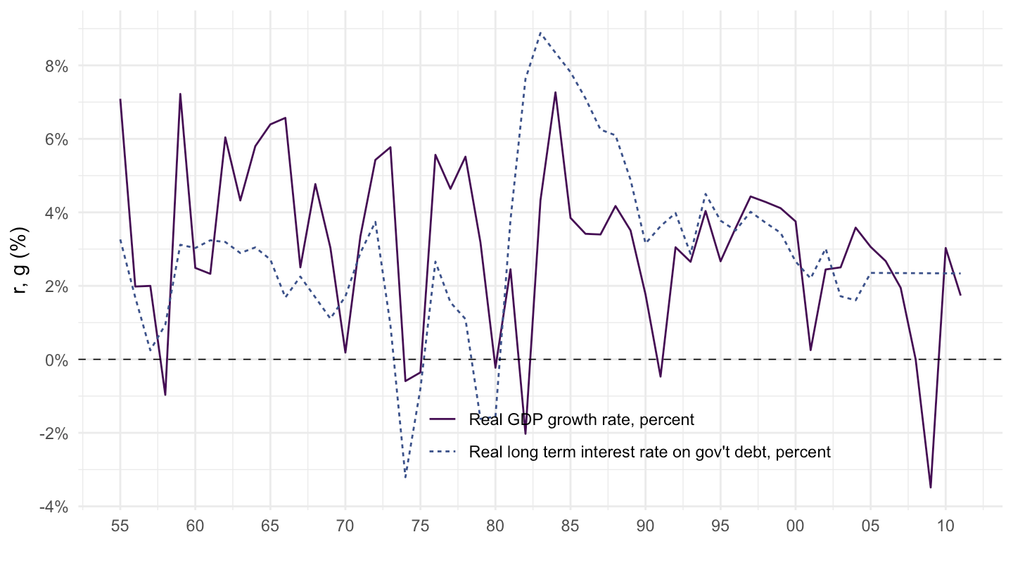

Ex 7: Regressions

r on g

Code

data <- MauroRomeuBinderZaman2013 |>
  filter(variable %in% c("rgc", "rltirc")) |>
  spread(variable, value) |>
  rename(g = rgc, r = rltirc) |>
  group_by(iso2c) |>
  mutate(r = forecast::ma(r, 5),
         g = forecast::ma(g, 5),
         r = r/100,
         g = g/100,
         `r-g` = r-g,
         g_lead1 = lead(g, 1),
         g_lead2 = lead(g, 2),
         g_lead3 = lead(g, 3)) |>
  na.omit() |>
  filter(abs(r) <0.5, abs(g) <0.5)

Code

data %>%
  lm(r ~ g, data = .) |>
  summary()

# 
# Call:
# lm(formula = r ~ g, data = .)
# 
# Residuals:
#      Min       1Q   Median       3Q      Max 
# -0.33076 -0.01445  0.00251  0.02221  0.12083 
# 
# Coefficients:
#              Estimate Std. Error t value Pr(>|t|)    
# (Intercept)  0.030177   0.001486  20.307   <2e-16 ***
# g           -0.089797   0.039322  -2.284   0.0225 *  
# ---
# Signif. codes:  0 '***' 0.001 '**' 0.01 '*' 0.05 '.' 0.1 ' ' 1
# 
# Residual standard error: 0.03874 on 1884 degrees of freedom
# Multiple R-squared:  0.00276, Adjusted R-squared:  0.002231 
# F-statistic: 5.215 on 1 and 1884 DF,  p-value: 0.0225

Code

data %>%
  lm(r ~ g_lead1 + g_lead2 + g_lead3, data = .) |>
  summary()

# 
# Call:
# lm(formula = r ~ g_lead1 + g_lead2 + g_lead3, data = .)
# 
# Residuals:
#      Min       1Q   Median       3Q      Max 
# -0.32558 -0.01481  0.00265  0.02244  0.11906 
# 
# Coefficients:
#              Estimate Std. Error t value Pr(>|t|)    
# (Intercept)  0.026967   0.001549  17.407  < 2e-16 ***
# g_lead1     -0.224180   0.079430  -2.822  0.00482 ** 
# g_lead2      0.215701   0.116800   1.847  0.06494 .  
# g_lead3      0.030538   0.078554   0.389  0.69750    
# ---
# Signif. codes:  0 '***' 0.001 '**' 0.01 '*' 0.05 '.' 0.1 ' ' 1
# 
# Residual standard error: 0.0387 on 1882 degrees of freedom
# Multiple R-squared:  0.006183,    Adjusted R-squared:  0.004599 
# F-statistic: 3.903 on 3 and 1882 DF,  p-value: 0.008582

Code

data |>
  ggplot() + geom_point(aes(g, r)) + theme_minimal() +
  xlab("g (%)") + ylab("r (%)") +
  scale_x_continuous(breaks = 0.01*seq(-100, 200, 10),
                     labels = scales::percent_format(accuracy = 1)) +
  scale_y_continuous(breaks = 0.01*seq(-100, 200, 10),
                     labels = scales::percent_format(accuracy = 1)) +
  stat_smooth(aes(g, r), linetype = 2,  method = "lm", color = viridis(3)[2])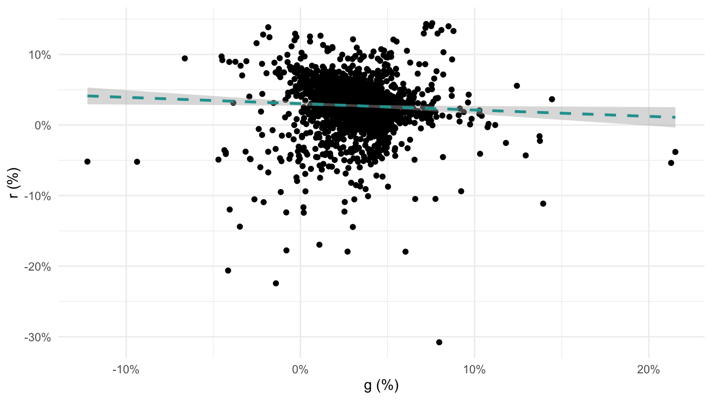

Code

library(ggplot2)
library(ggpmisc)
df <- data.frame(x = c(1:100))
df$y <- 2 + 3 * df$x + rnorm(100, sd = 40)
my.formula <- y ~ x
p <- ggplot(data = df, aes(x = x, y = y)) +
   geom_smooth(method = "lm", se=FALSE, color="black", formula = my.formula) +
   stat_poly_eq(formula = my.formula, 
                aes(label = paste(..eq.label.., ..rr.label.., sep = "~~~")), 
                parse = TRUE) +         
   geom_point()
p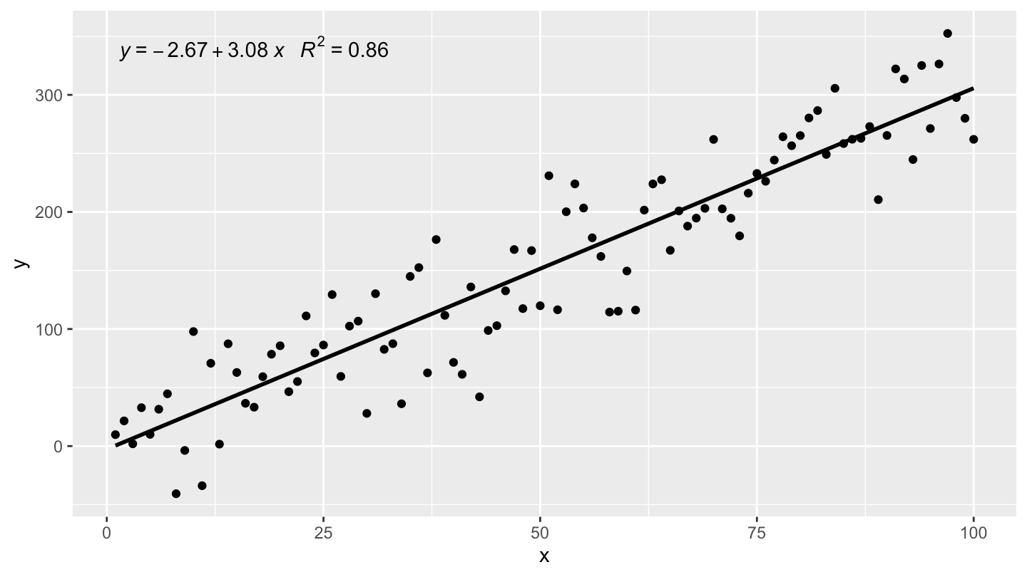

r-g on r

Code

data %>%
  lm(`r-g` ~ r, data = .) |>
  summary()

# 
# Call:
# lm(formula = `r-g` ~ r, data = .)
# 
# Residuals:
#       Min        1Q    Median        3Q       Max 
# -0.183010 -0.011815  0.001134  0.012313  0.154911 
# 
# Coefficients:
#               Estimate Std. Error t value Pr(>|t|)    
# (Intercept) -0.0310681  0.0006396  -48.57   <2e-16 ***
# r            1.0307410  0.0134613   76.57   <2e-16 ***
# ---
# Signif. codes:  0 '***' 0.001 '**' 0.01 '*' 0.05 '.' 0.1 ' ' 1
# 
# Residual standard error: 0.02267 on 1884 degrees of freedom
# Multiple R-squared:  0.7568,  Adjusted R-squared:  0.7567 
# F-statistic:  5863 on 1 and 1884 DF,  p-value: < 2.2e-16

Code

data |>
  ggplot() + geom_point(aes(r, r-g)) + theme_minimal() +
  xlab("r (%)") + ylab("r-g (%)") +
  scale_x_continuous(breaks = 0.01*seq(-100, 200, 10),
                     labels = scales::percent_format(accuracy = 1)) +
  scale_y_continuous(breaks = 0.01*seq(-100, 200, 10),
                     labels = scales::percent_format(accuracy = 1)) +
  stat_smooth(aes(r, r-g), linetype = 2,  method = "lm", color = viridis(3)[2])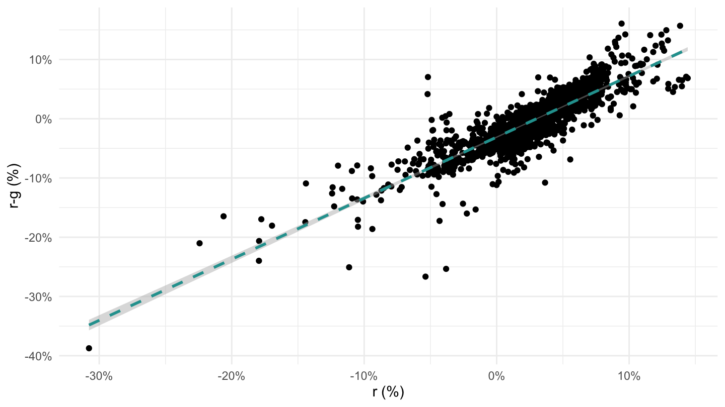

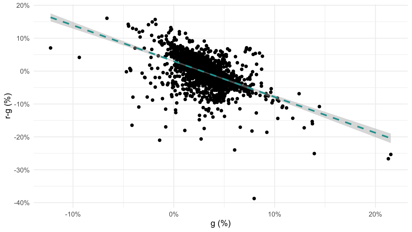
r-g on g

Code

data %>%
  lm(`r-g` ~ g, data = .) |>
  summary()

# 
# Call:
# lm(formula = `r-g` ~ g, data = .)
# 
# Residuals:
#      Min       1Q   Median       3Q      Max 
# -0.33076 -0.01445  0.00251  0.02221  0.12083 
# 
# Coefficients:
#              Estimate Std. Error t value Pr(>|t|)    
# (Intercept)  0.030177   0.001486   20.31   <2e-16 ***
# g           -1.089797   0.039322  -27.71   <2e-16 ***
# ---
# Signif. codes:  0 '***' 0.001 '**' 0.01 '*' 0.05 '.' 0.1 ' ' 1
# 
# Residual standard error: 0.03874 on 1884 degrees of freedom
# Multiple R-squared:  0.2896,  Adjusted R-squared:  0.2892 
# F-statistic: 768.1 on 1 and 1884 DF,  p-value: < 2.2e-16

Code

data |>
  ggplot() + geom_point(aes(g, r-g)) + theme_minimal() +
  xlab("g (%)") + ylab("r-g (%)") +
  scale_x_continuous(breaks = 0.01*seq(-100, 200, 10),
                     labels = scales::percent_format(accuracy = 1)) +
  scale_y_continuous(breaks = 0.01*seq(-100, 200, 10),
                     labels = scales::percent_format(accuracy = 1)) +
  stat_smooth(aes(g, r-g), linetype = 2,  method = "lm", color = viridis(3)[2])