Code
GFSE %>%
  left_join(INDICATOR, by = "INDICATOR") %>%
  group_by(INDICATOR, Indicator) %>%
  summarise(Nobs = n()) %>%
  arrange(-Nobs) %>%
{if (is_html_output()) datatable(., filter = 'top', rownames = F) else .}Data - IMF
GFSE %>%
left_join(INDICATOR, by = "INDICATOR") %>%
group_by(INDICATOR, Indicator) %>%
summarise(Nobs = n()) %>%
arrange(-Nobs) %>%
{if (is_html_output()) datatable(., filter = 'top', rownames = F) else .}GFSE %>%
left_join(SECTOR, by = "SECTOR") %>%
group_by(SECTOR, Sector) %>%
summarise(Nobs = n()) %>%
arrange(-Nobs) %>%
{if (is_html_output()) print_table(.) else .}| SECTOR | Sector | Nobs |
|---|---|---|
| S1311B | Budgetary central government | 176362 |
| S1321 | Central government (incl. social security funds) | 136991 |
| S1311 | Central government (excl. social security funds) | 119075 |
| S13 | General government | 115125 |
| S1314 | Social security funds | 112229 |
| S1313 | Local governments | 108804 |
| S13112 | Extrabudgetary central government | 67887 |
| S1312 | State governments | 34689 |
GFSE %>%
  left_join(iso2c, by = "iso2c") %>%
  group_by(iso2c, Iso2c) %>%
  summarise(Nobs = n()) %>%
  arrange(-Nobs) %>%
{if (is_html_output()) datatable(., filter = 'top', rownames = F) else .}GFSE %>%
group_by(CLASSIFICATION) %>%
summarise(Nobs = n()) %>%
arrange(-Nobs) %>%
{if (is_html_output()) datatable(., filter = 'top', rownames = F) else .}GFSE %>%
left_join(CL_UNIT_GFSE, by = "UNIT") %>%
group_by(UNIT, UNIT_desc) %>%
summarise(Nobs = n()) %>%
arrange(-Nobs) %>%
{if (is_html_output()) print_table(.) else .}| UNIT | UNIT_desc | Nobs |
|---|---|---|
| XDC | Domestic currency | 436756 |
| XDC_R_B1GQ | Percent of GDP | 434406 |
GFSE %>%
  left_join(SECTOR, by = "SECTOR") %>%
  left_join(iso2c, by = "iso2c") %>%
  filter(INDICATOR == "W0_S1_G24",
         UNIT == "XDC_R_B1GQ",
         SECTOR == "S1321") %>%
  group_by(iso2c, Iso2c) %>%
  summarise(Nobs = n(),
            year1 = first(year(date)),
            value1 = first(round(value, 1)),
            year2 = last(year(date)),
            value2 = last(round(value, 1))) %>%
  arrange(-Nobs) %>%
{if (is_html_output()) datatable(., filter = 'top', rownames = F) else .}GFSE %>%
left_join(iso2c, by = "iso2c") %>%
filter(INDICATOR == "W0_S1_G24",
UNIT == "XDC_R_B1GQ",
iso2c %in% c("AT", "AU", "CY"),
SECTOR == "S1321") %>%
ggplot(.) + geom_line(aes(x = date, y = value/100, color = Iso2c)) + theme_minimal() +
xlab("") + ylab("Interest Payments (% of GDP)") +
scale_color_manual(values = c("#00008B", "#ED2939", "#D47600")) +
theme(legend.title = element_blank(),
legend.position = c(0.15, 0.85)) +
scale_x_date(breaks = seq(1900, 2020, 5) %>% paste0("-01-01") %>% as.Date,
labels = date_format("%y")) +
geom_image(data = . %>%
filter(date == as.Date("2018-12-31")) %>%
mutate(image = paste0("../../icon/flag/", str_to_lower(gsub(" ", "-", Iso2c)), ".png")),
aes(x = date, y = value/100, image = image), asp = 1.5) +
scale_y_continuous(breaks = 0.01*seq(-100, 10000, 1),
labels = percent_format(a = 1)) +
geom_hline(yintercept = 0, linetype = "dashed", color = "grey")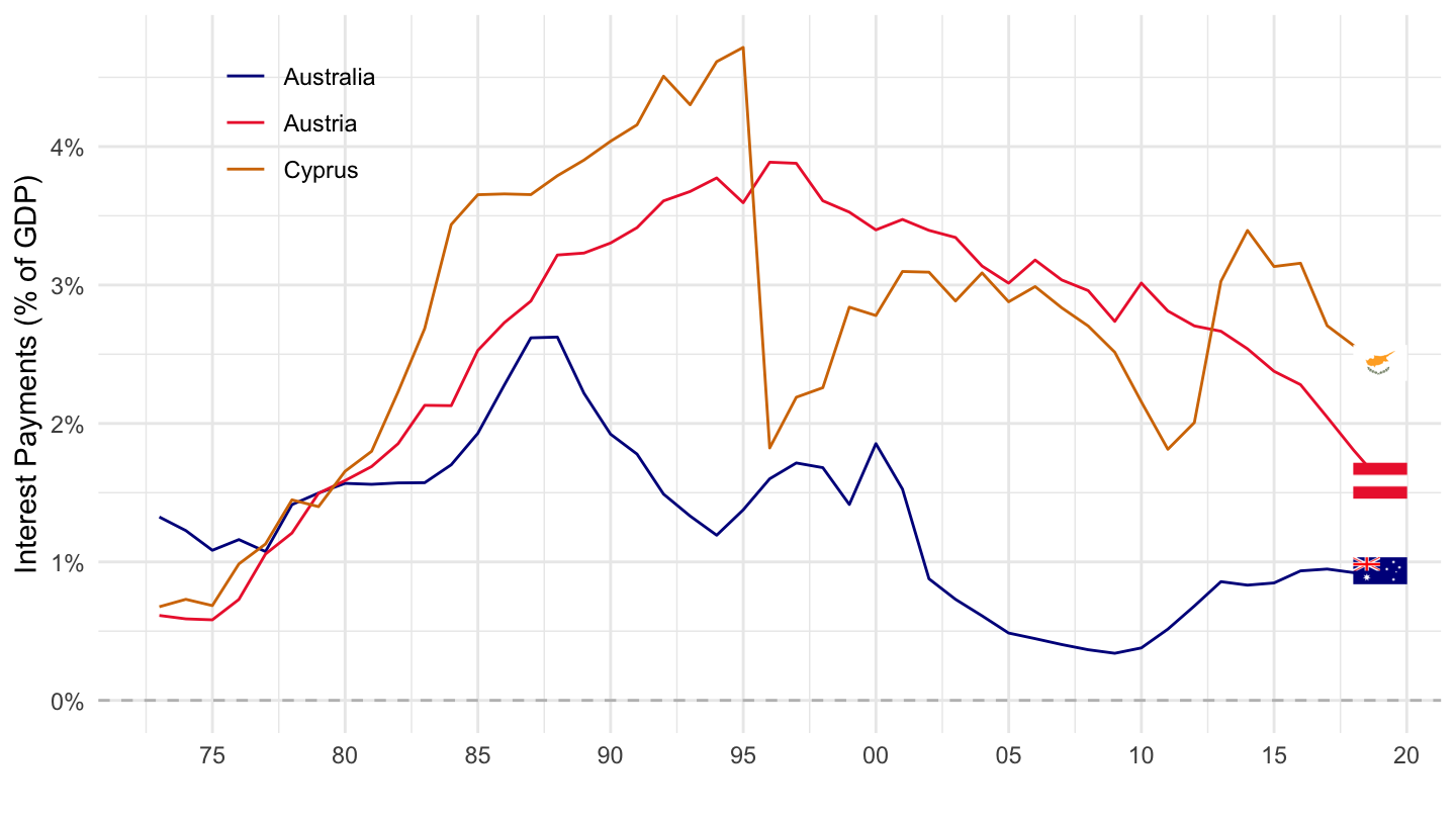
GFSE %>%
  left_join(iso2c, by = "iso2c") %>%
  filter(INDICATOR == "W0_S1_G24",
         UNIT == "XDC_R_B1GQ",
         iso2c %in% c("DE", "FR", "IT"),
         SECTOR == "S1321") %>%
  ggplot(.) + geom_line(aes(x = date, y = value/100, color = Iso2c)) + theme_minimal() +
  xlab("") + ylab("Interest Payments (% of GDP)") +
  scale_color_manual(values = c("#002395", "#000000", "#009246")) +
  theme(legend.title = element_blank(),
        legend.position = c(0.15, 0.85)) +
  geom_image(data = . %>%
               filter(date == as.Date("2018-12-31")) %>%
               mutate(image = paste0("../../icon/flag/", str_to_lower(gsub(" ", "-", Iso2c)), ".png")),
             aes(x = date, y = value/100, image = image), asp = 1.5) +
  scale_x_date(breaks = seq(1900, 2020, 5) %>% paste0("-01-01") %>% as.Date,
               labels = date_format("%y")) +
  scale_y_continuous(breaks = 0.01*seq(-100, 10000, 1),
                     labels = percent_format(a = 1)) +
  geom_hline(yintercept = 0, linetype = "dashed", color = "grey")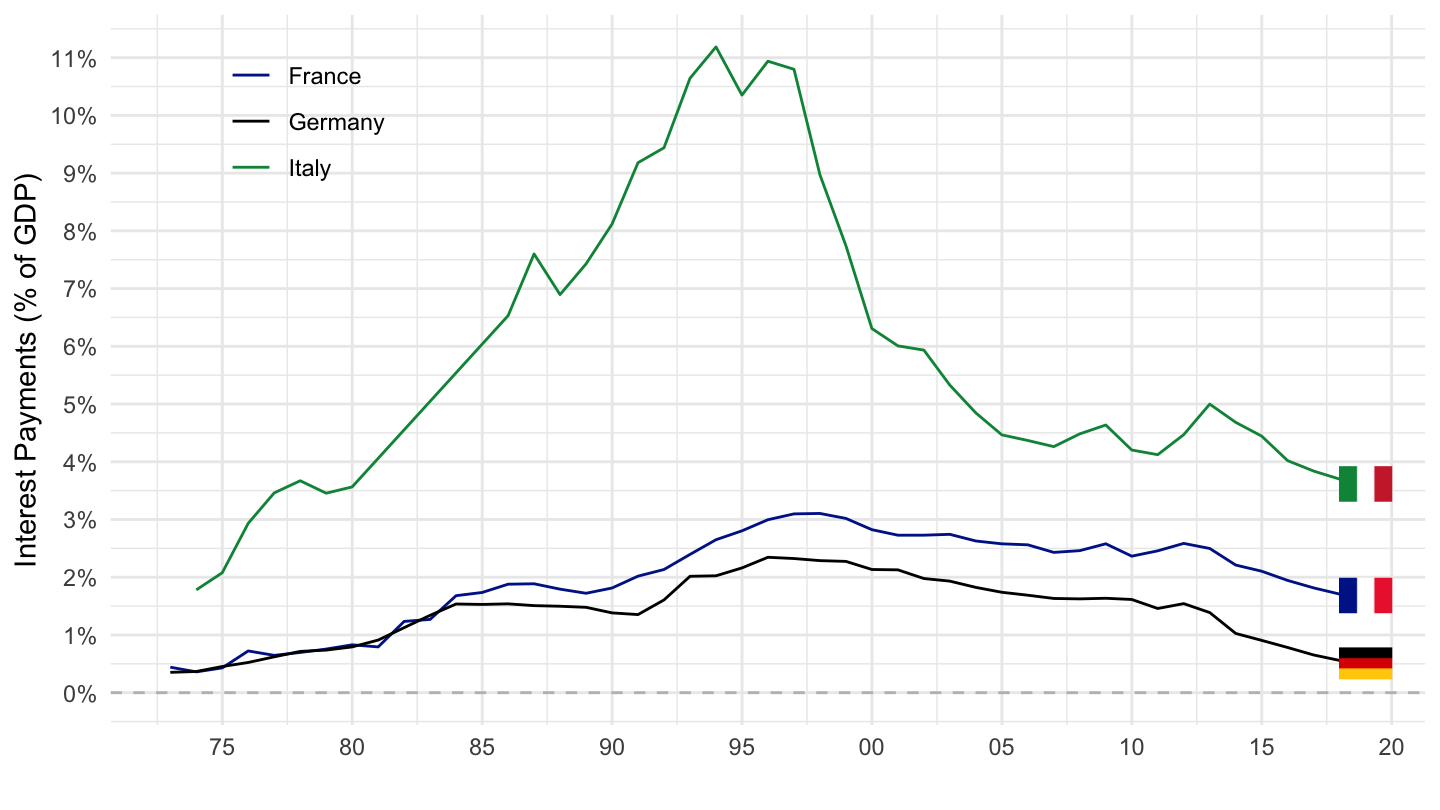
GFSE %>%
  left_join(iso2c, by = "iso2c") %>%
  filter(INDICATOR == "W0_S1_G24",
         UNIT == "XDC_R_B1GQ",
         iso2c %in% c("GB", "IE", "US"),
         SECTOR == "S1321") %>%
  ggplot(.) + geom_line(aes(x = date, y = value/100, color = Iso2c)) + theme_minimal() +
  xlab("") + ylab("Interest Payments (% of GDP)") +
  scale_color_manual(values = c("#169B62", "#6E82B5", "#B22234")) +
  theme(legend.title = element_blank(),
        legend.position = c(0.85, 0.85)) +
  scale_x_date(breaks = seq(1900, 2020, 5) %>% paste0("-01-01") %>% as.Date,
               labels = date_format("%y")) +
  scale_y_continuous(breaks = 0.01*seq(-100, 10000, 1),
                     labels = percent_format(a = 1)) +
  geom_image(data = . %>%
               filter(date == as.Date("2006-12-31")) %>%
               mutate(image = paste0("../../icon/flag/", str_to_lower(gsub(" ", "-", Iso2c)), ".png")),
             aes(x = date, y = value/100, image = image), asp = 1.5) +
  geom_hline(yintercept = 0, linetype = "dashed", color = "grey")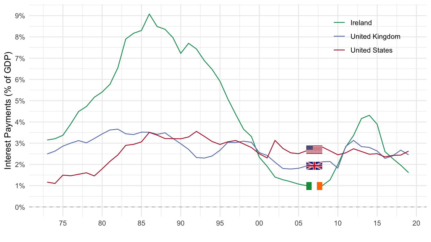
GFSE %>%
  left_join(SECTOR, by = "SECTOR") %>%
  left_join(iso2c, by = "iso2c") %>%
  filter(INDICATOR == "W1_S1_G24",
         UNIT == "XDC_R_B1GQ",
         SECTOR == "S1321") %>%
  group_by(iso2c, Iso2c) %>%
  summarise(Nobs = n(),
            year1 = first(year(date)),
            value1 = first(round(value, 1)),
            year2 = last(year(date)),
            value2 = last(round(value, 1))) %>%
  arrange(-Nobs) %>%
{if (is_html_output()) datatable(., filter = 'top', rownames = F) else .}GFSE %>%
left_join(iso2c, by = "iso2c") %>%
filter(INDICATOR == "W1_S1_G24",
UNIT == "XDC_R_B1GQ",
iso2c %in% c("CG", "KI", "SV"),
SECTOR == "S1321") %>%
ggplot(.) + geom_line() + theme_minimal() +
aes(x = date, y = value/100, color = Iso2c, linetype = Iso2c) +
xlab("") + ylab("Interest Payments to Non Residents (% of GDP)") +
scale_color_manual(values = viridis(4)[1:3]) +
theme(legend.title = element_blank(),
legend.position = c(0.85, 0.85)) +
scale_x_date(breaks = seq(1900, 2020, 2) %>% paste0("-01-01") %>% as.Date,
labels = date_format("%y")) +
scale_y_continuous(breaks = 0.01*seq(-100, 10000, 1),
labels = percent_format(a = 1)) +
geom_hline(yintercept = 0, linetype = "dashed", color = "grey")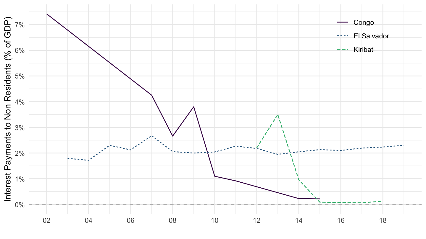
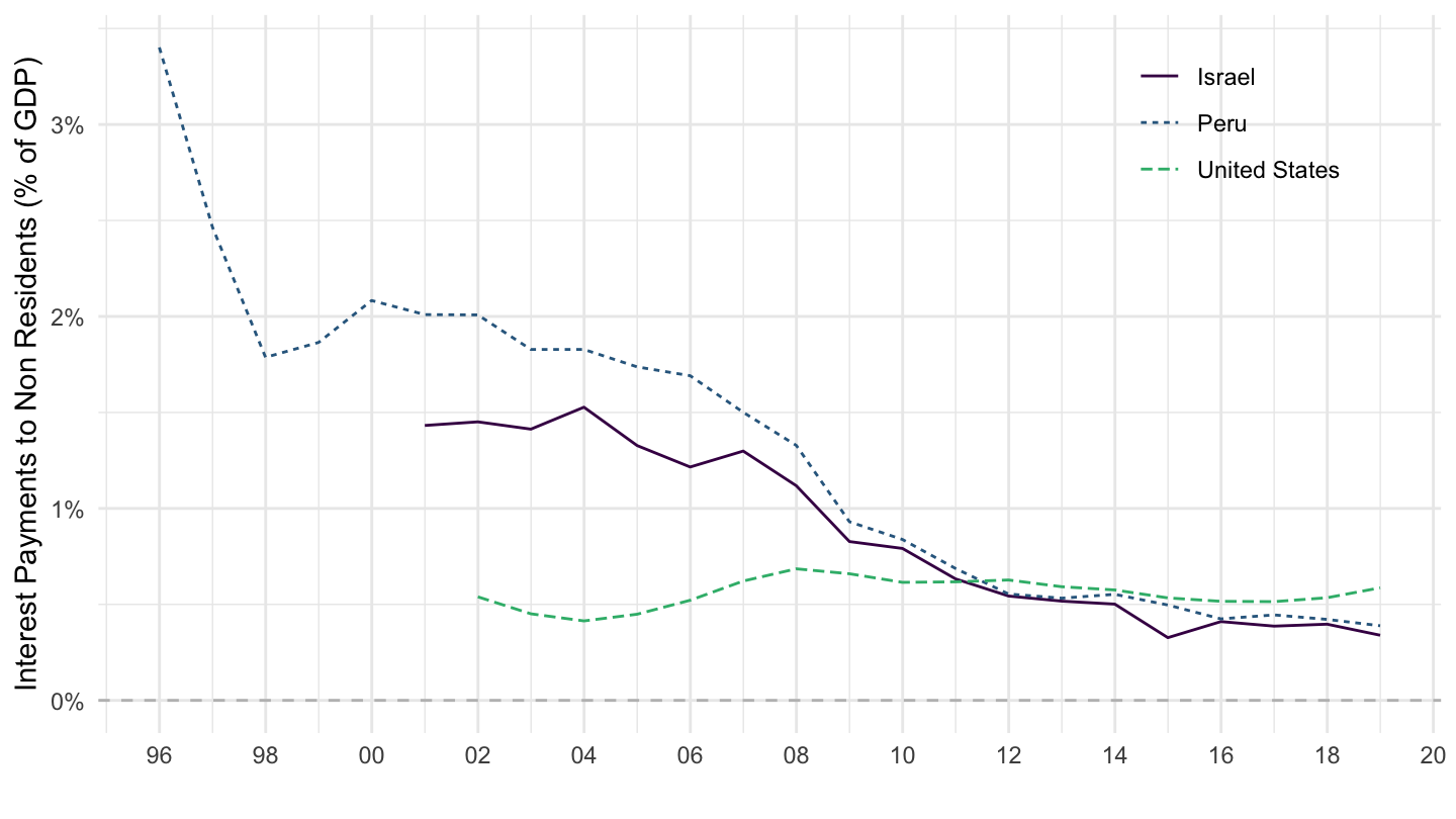
GFSE %>%
  left_join(iso2c, by = "iso2c") %>%
  filter(INDICATOR == "W1_S1_G24",
         UNIT == "XDC_R_B1GQ",
         iso2c %in% c("US", "PE", "IL"),
         SECTOR == "S1321") %>%
  ggplot(.) + geom_line() + theme_minimal() +
  aes(x = date, y = value/100, color = Iso2c, linetype = Iso2c) +
  xlab("") + ylab("Interest Payments to Non Residents (% of GDP)") +
  scale_color_manual(values = viridis(4)[1:3]) +
  theme(legend.title = element_blank(),
        legend.position = c(0.85, 0.85)) +
  scale_x_date(breaks = seq(1900, 2020, 2) %>% paste0("-01-01") %>% as.Date,
               labels = date_format("%y")) +
  scale_y_continuous(breaks = 0.01*seq(-100, 10000, 1),
                     labels = percent_format(a = 1)) +
  geom_hline(yintercept = 0, linetype = "dashed", color = "grey")