Code
tibble(DOWNLOAD_TIME = as.Date(file.info("~/iCloud/website/data/imf/DOT_CN.RData")$mtime)) %>%
print_table_conditional()| DOWNLOAD_TIME |
|---|
| 2025-01-05 |
Data - IMF
tibble(DOWNLOAD_TIME = as.Date(file.info("~/iCloud/website/data/imf/DOT_CN.RData")$mtime)) %>%
print_table_conditional()| DOWNLOAD_TIME |
|---|
| 2025-01-05 |
DOT_CN %>%
  group_by(TIME_PERIOD) %>%
  summarise(Nobs = n()) %>%
  arrange(desc(TIME_PERIOD)) %>%
  head(1) %>%
print_table_conditional()| TIME_PERIOD | Nobs |
|---|---|
| 2024-Q3 | 694 |
DOT_CN %>%
  left_join(FREQ, by = "FREQ") %>%
  group_by(FREQ, Freq) %>%
  summarise(Nobs = n()) %>%
  arrange(-Nobs) %>%
{if (is_html_output()) print_table(.) else .}| FREQ | Freq | Nobs |
|---|---|---|
| M | Monthly | 297625 |
| Q | Quarterly | 102870 |
| A | Annual | 26976 |
DOT_CN %>%
  left_join(INDICATOR, by = "INDICATOR") %>%
  group_by(INDICATOR, Indicator) %>%
  summarise(Nobs = n()) %>%
  arrange(-Nobs) %>%
{if (is_html_output()) print_table(.) else .}| INDICATOR | Indicator | Nobs |
|---|---|---|
| TBG_USD | Goods, Value of Trade Balance, US Dollars | 151495 |
| TXG_FOB_USD | Goods, Value of Exports, Free on board (FOB), US Dollars | 149810 |
| TMG_CIF_USD | Goods, Value of Imports, Cost, Insurance, Freight (CIF), US Dollars | 126166 |
DOT_CN %>%
  left_join(COUNTERPART_AREA, by = "COUNTERPART_AREA") %>%
  group_by(COUNTERPART_AREA, Counterpart_area) %>%
  summarise(Nobs = n()) %>%
  arrange(-Nobs) %>%
  mutate(Flag = gsub(" ", "-", str_to_lower(gsub(" ", "-", Counterpart_area))),
         Flag = paste0('<img src="../../icon/flag/vsmall/', Flag, '.png" alt="Flag">')) %>%
  select(Flag, everything()) %>%
{if (is_html_output()) datatable(., filter = 'top', rownames = F, escape = F) else .}DOT_CN %>%
group_by(TIME_PERIOD) %>%
summarise(Nobs = n()) %>%
arrange(desc(TIME_PERIOD)) %>%
slice(1:10, (n()-10):n()) %>%
print_table_conditional()| TIME_PERIOD | Nobs |
|---|---|
| 2024-Q3 | 694 |
| 2024-Q2 | 691 |
| 2024-Q1 | 694 |
| 2024-09 | 687 |
| 2024-08 | 690 |
| 2024-07 | 686 |
| 2024-06 | 688 |
| 2024-05 | 683 |
| 2024-04 | 687 |
| 2024-03 | 684 |
| 1961-10 | 24 |
| 1961-09 | 24 |
| 1961-08 | 24 |
| 1961-07 | 24 |
| 1961-06 | 24 |
| 1961-05 | 24 |
| 1961-04 | 24 |
| 1961-03 | 24 |
| 1961-02 | 24 |
| 1961-01 | 24 |
| 1961 | 184 |
DOT_CN %>%
  filter(COUNTERPART_AREA %in% c("DE", "FR", "U2", "US", "E1", "B0"),
         FREQ == "Q",
         INDICATOR == "TBG_USD") %>%
  mutate(OBS_VALUE = OBS_VALUE*10^(UNIT_MULT)) %>%
  left_join(INDICATOR, by = "INDICATOR") %>%
  quarter_to_date2 %>%
  left_join(COUNTERPART_AREA, by = "COUNTERPART_AREA") %>%
  left_join(colors, by = c("Counterpart_area" = "country")) %>%
  ggplot + geom_line(aes(x = date, y = OBS_VALUE, color = color)) +
  scale_color_identity() + add_flags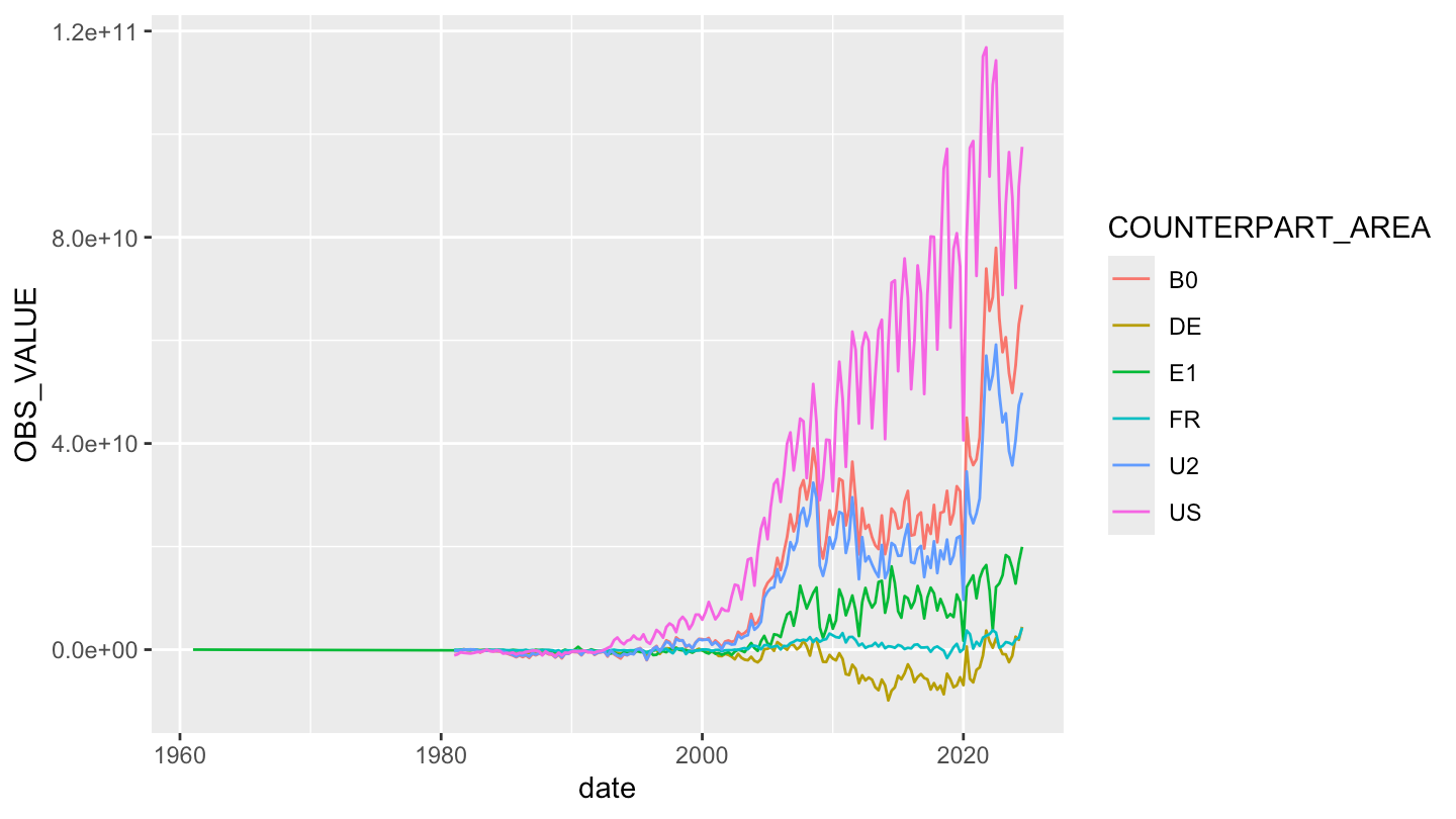
DOT_CN %>%
  filter(COUNTERPART_AREA %in% c("DE", "FR", "U2", "US"),
         FREQ == "Q",
         INDICATOR == "TBG_USD") %>%
  mutate(OBS_VALUE = OBS_VALUE*10^(UNIT_MULT)) %>%
  left_join(INDICATOR, by = "INDICATOR") %>%
  quarter_to_date2 %>%
  left_join(COUNTERPART_AREA, by = "COUNTERPART_AREA") %>%
  left_join(colors, by = c("Counterpart_area" = "country")) %>%
  ggplot + geom_line(aes(x = date, y = OBS_VALUE, color = color)) +
  scale_color_identity() + add_flags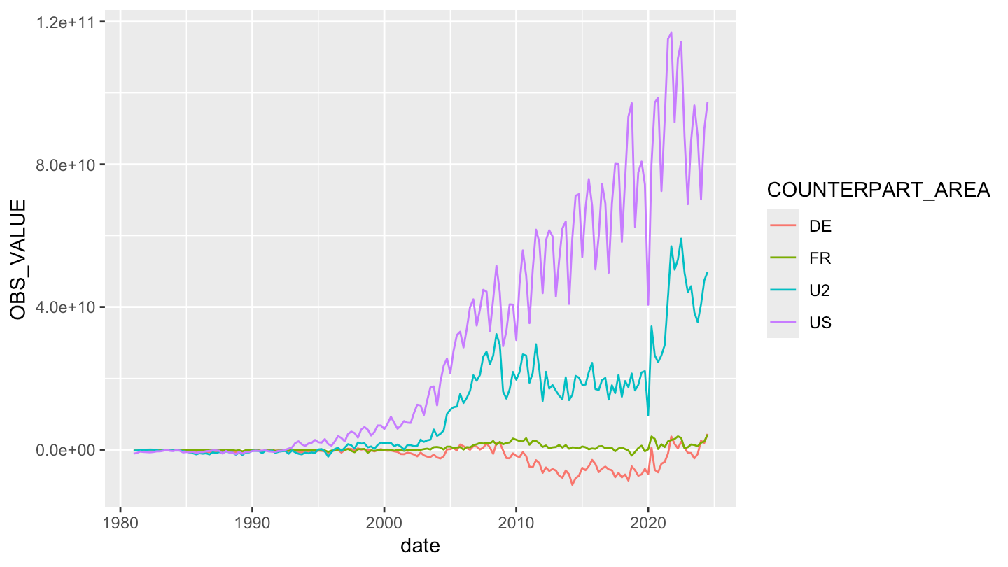
DOT_CN %>%
  filter(COUNTERPART_AREA == "DE",
         FREQ == "A") %>%
  mutate(OBS_VALUE = OBS_VALUE*10^(UNIT_MULT)) %>%
  left_join(INDICATOR, by = "INDICATOR") %>%
  select(TIME_PERIOD, Indicator, OBS_VALUE) %>%
  spread(Indicator, OBS_VALUE) %>%
  arrange(desc(TIME_PERIOD)) %>%
print_table_conditional()DOT_CN %>%
filter(COUNTERPART_AREA == "DE",
FREQ == "Q",
INDICATOR == "TBG_USD") %>%
mutate(OBS_VALUE = OBS_VALUE*10^(UNIT_MULT)) %>%
left_join(INDICATOR, by = "INDICATOR") %>%
select(TIME_PERIOD, Indicator, OBS_VALUE) %>%
quarter_to_date2 %>%
ggplot + geom_line(aes(x = date, y = OBS_VALUE))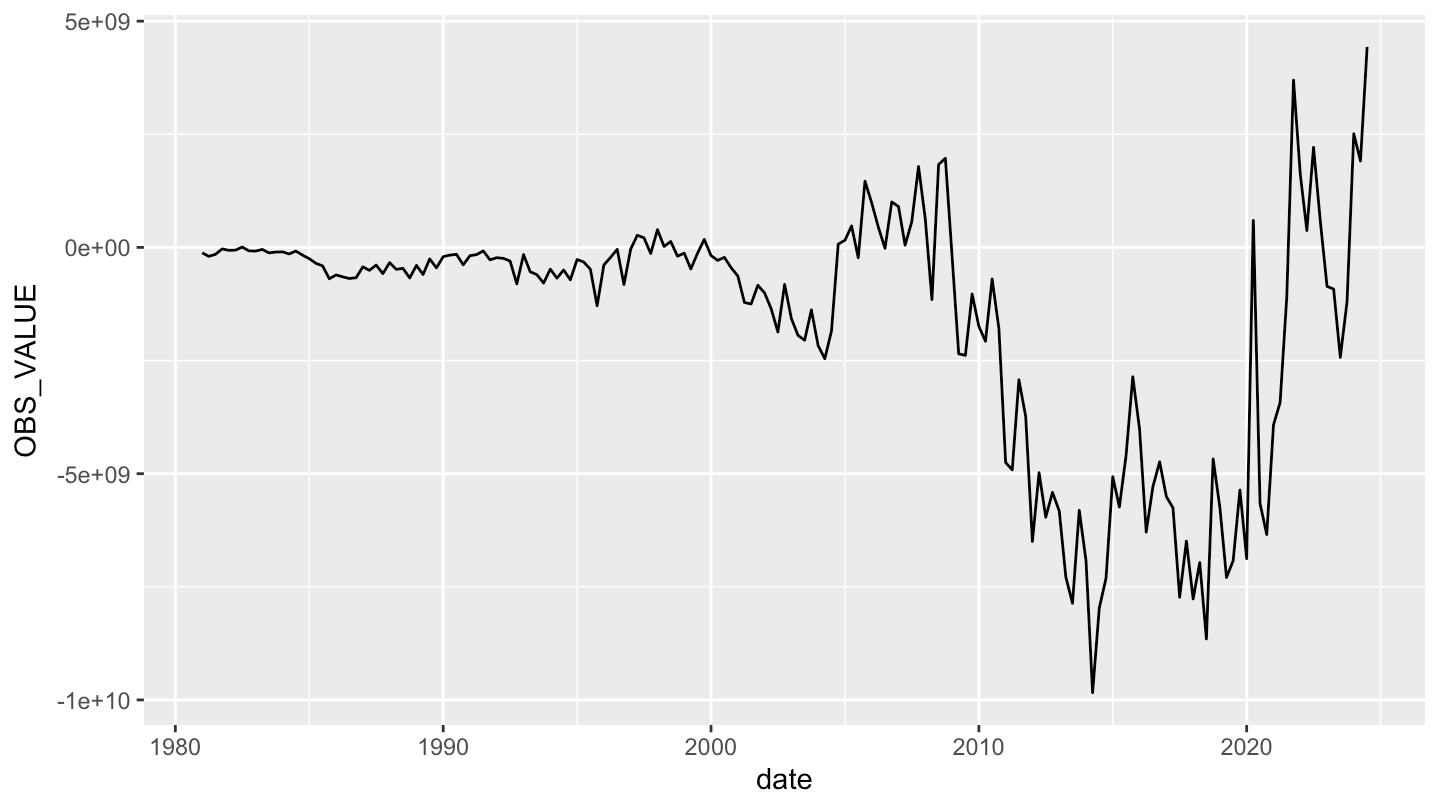
DOT_CN %>%
  filter(COUNTERPART_AREA == "DE",
         FREQ == "Q") %>%
  mutate(OBS_VALUE = OBS_VALUE*10^(UNIT_MULT)) %>%
  left_join(INDICATOR, by = "INDICATOR") %>%
  select(TIME_PERIOD, Indicator, OBS_VALUE) %>%
  spread(Indicator, OBS_VALUE) %>%
  arrange(desc(TIME_PERIOD)) %>%
print_table_conditional()DOT_CN %>%
filter(COUNTERPART_AREA == "DE",
FREQ == "M",
INDICATOR == "TBG_USD") %>%
mutate(OBS_VALUE = OBS_VALUE*10^(UNIT_MULT)) %>%
left_join(INDICATOR, by = "INDICATOR") %>%
select(TIME_PERIOD, Indicator, OBS_VALUE) %>%
month_to_date2 %>%
ggplot + geom_line(aes(x = date, y = OBS_VALUE))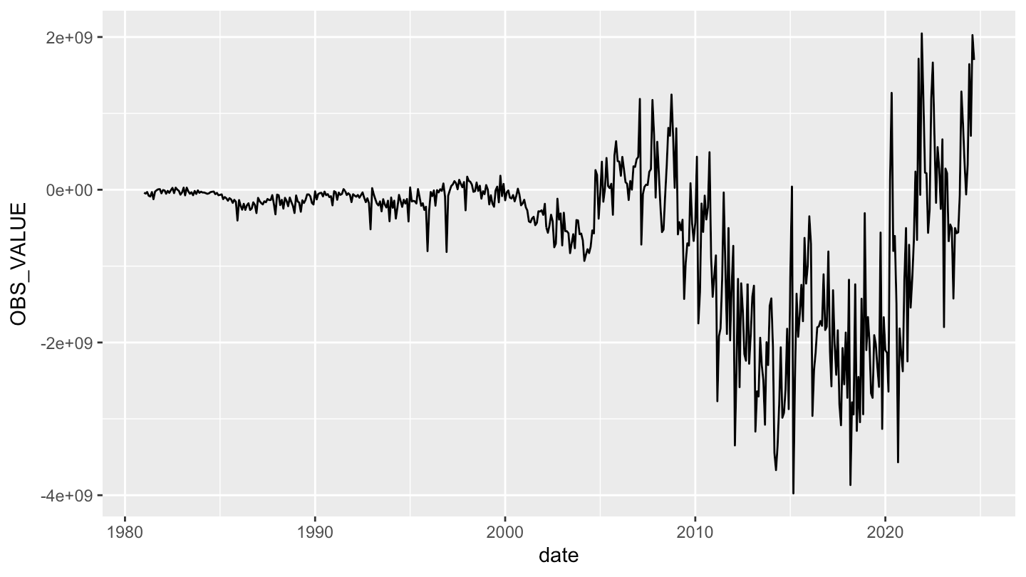
DOT_CN %>%
  filter(COUNTERPART_AREA == "DE",
         FREQ == "M") %>%
  mutate(OBS_VALUE = OBS_VALUE*10^(UNIT_MULT)) %>%
  left_join(INDICATOR, by = "INDICATOR") %>%
  select(TIME_PERIOD, Indicator, OBS_VALUE) %>%
  spread(Indicator, OBS_VALUE) %>%
  arrange(desc(TIME_PERIOD)) %>%
print_table_conditional()DOT_CN %>%
left_join(NGDP_USD %>%
select(FREQ, REF_AREA, TIME_PERIOD, NGDP_USD = OBS_VALUE),
by = c("TIME_PERIOD", "REF_AREA", "FREQ")) %>%
filter(TIME_PERIOD %in% c("2019", "2010", "2000", "1990"),
INDICATOR == "TBG_USD") %>%
mutate(OBS_VALUE = OBS_VALUE*10^(UNIT_MULT)/NGDP_USD) %>%
left_join(COUNTERPART_AREA, by = "COUNTERPART_AREA") %>%
select(COUNTERPART_AREA, Counterpart_area, TIME_PERIOD, OBS_VALUE) %>%
spread(TIME_PERIOD, OBS_VALUE) %>%
arrange(-`2019`) %>%
mutate_at(vars(-1, -2), funs(round(100*., 2))) %>%
mutate(Flag = gsub(" ", "-", str_to_lower(gsub(" ", "-", Counterpart_area))),
Flag = paste0('<img src="../../icon/flag/vsmall/', Flag, '.png" alt="Flag">')) %>%
select(Flag, everything()) %>%
{if (is_html_output()) datatable(., filter = 'top', rownames = F, escape = F) else .}DOT_CN %>%
left_join(NGDP_USD %>%
select(FREQ, REF_AREA, TIME_PERIOD, NGDP_USD = OBS_VALUE),
by = c("TIME_PERIOD", "REF_AREA", "FREQ")) %>%
filter(TIME_PERIOD %in% c("2019", "2010", "2000", "1990"),
INDICATOR == "TBG_USD") %>%
mutate(OBS_VALUE = OBS_VALUE*10^(UNIT_MULT)/NGDP_USD) %>%
left_join(COUNTERPART_AREA, by = "COUNTERPART_AREA") %>%
select(COUNTERPART_AREA, Counterpart_area, TIME_PERIOD, OBS_VALUE) %>%
spread(TIME_PERIOD, OBS_VALUE) %>%
arrange(-`2019`) %>%
mutate_at(vars(-1, -2), funs(round(100*., 2))) %>%
filter(!is.na(`2019`),
`2019` > 0.04) %>%
mutate(Flag = gsub(" ", "-", str_to_lower(gsub(" ", "-", Counterpart_area))),
Flag = paste0('<img src="../../icon/flag/vsmall/', Flag, '.png" alt="Flag">')) %>%
select(Flag, everything()) %>%
{if (is_html_output()) datatable(., filter = 'top', rownames = F, escape = F) else .}DOT_CN %>%
left_join(NGDP_USD %>%
select(FREQ, REF_AREA, TIME_PERIOD, NGDP_USD = OBS_VALUE),
by = c("TIME_PERIOD", "REF_AREA", "FREQ")) %>%
filter(TIME_PERIOD %in% c("2019", "2010", "2000", "1990"),
INDICATOR == "TBG_USD") %>%
mutate(OBS_VALUE = OBS_VALUE*10^(UNIT_MULT)/NGDP_USD) %>%
left_join(COUNTERPART_AREA, by = "COUNTERPART_AREA") %>%
select(COUNTERPART_AREA, Counterpart_area, TIME_PERIOD, OBS_VALUE) %>%
spread(TIME_PERIOD, OBS_VALUE) %>%
arrange(`2019`) %>%
mutate_at(vars(-1, -2), funs(round(100*., 2))) %>%
filter(!is.na(`2019`),
`2019` < -0.11) %>%
mutate(Flag = gsub(" ", "-", str_to_lower(gsub(" ", "-", Counterpart_area))),
Flag = paste0('<img src="../../icon/flag/vsmall/', Flag, '.png" alt="Flag">')) %>%
select(Flag, everything()) %>%
{if (is_html_output()) datatable(., filter = 'top', rownames = F, escape = F) else .}DOT_CN %>%
filter(COUNTERPART_AREA %in% c("GB", "US", "SG"),
INDICATOR %in% c("TBG_USD"),
FREQ == "A") %>%
inner_join(NGDP_USD %>%
filter(REF_AREA == "FR",
FREQ == "A") %>%
mutate(OBS_VALUE = OBS_VALUE*10^(UNIT_MULT)) %>%
select(TIME_PERIOD, NGDP_USD = OBS_VALUE),
by = "TIME_PERIOD") %>%
year_to_date2 %>%
mutate(OBS_VALUE = OBS_VALUE*10^(UNIT_MULT)/NGDP_USD) %>%
left_join(COUNTERPART_AREA, by = "COUNTERPART_AREA") %>%
mutate(Counterpart_area = ifelse(COUNTERPART_AREA == "U2", "Europe", Counterpart_area),
Counterpart_area = ifelse(COUNTERPART_AREA == "W00", "World", Counterpart_area)) %>%
left_join(colors, by = c("Counterpart_area" = "country")) %>%
mutate(color = ifelse(COUNTERPART_AREA == "DE", color2, color)) %>%
ggplot(.) + theme_minimal() + scale_color_identity() +
geom_line(aes(x = date, y = OBS_VALUE, color = color)) +
theme(legend.position = "none") + add_flags +
scale_x_date(breaks = seq(1950, 2100, 10) %>% paste0("-01-01") %>% as.Date,
labels = date_format("%Y")) +
scale_y_continuous(breaks = 0.01*seq(-500, 500, .1),
labels = percent_format(accuracy = .1)) +
xlab("") + ylab("China Bilateral Trade Surplus (% of GDP)") +
geom_hline(yintercept = 0, linetype = "dashed", color = "black")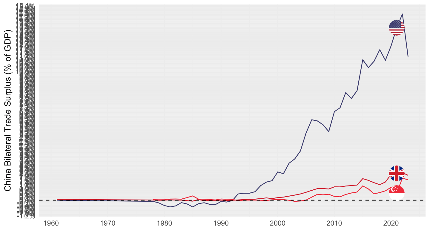
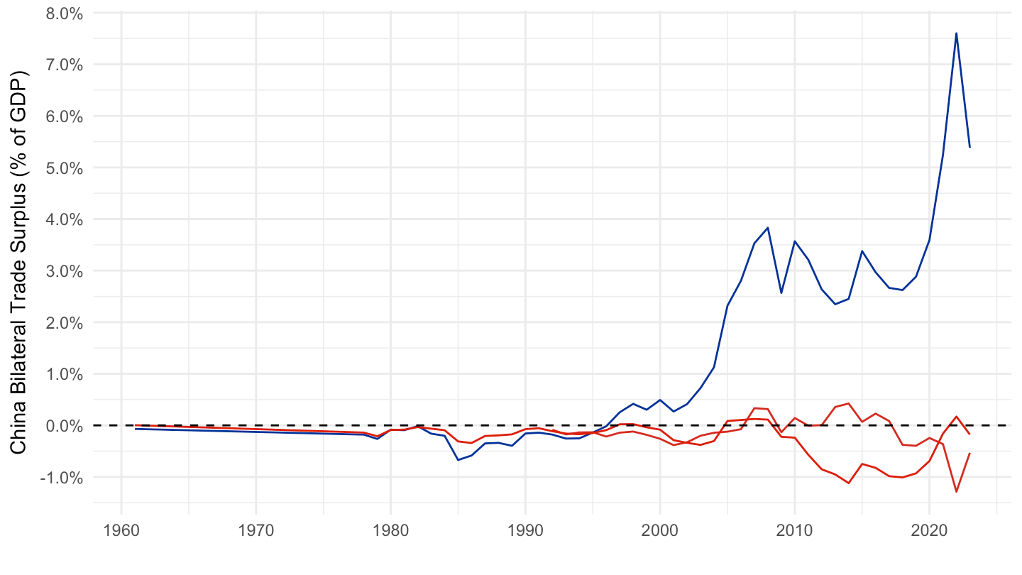
DOT_CN %>%
  filter(COUNTERPART_AREA  %in% c("QA", "HK", "EG"),
         INDICATOR %in% c("TBG_USD"),
         FREQ == "A") %>%
  inner_join(NGDP_USD %>%
              filter(REF_AREA == "FR",
                     FREQ == "A") %>%
              mutate(OBS_VALUE = OBS_VALUE*10^(UNIT_MULT)) %>%
              select(TIME_PERIOD, NGDP_USD = OBS_VALUE),
            by = "TIME_PERIOD") %>%
  year_to_date2 %>%
  mutate(OBS_VALUE = OBS_VALUE*10^(UNIT_MULT)/NGDP_USD) %>%
  left_join(COUNTERPART_AREA, by = "COUNTERPART_AREA") %>%
  mutate(Counterpart_area = ifelse(COUNTERPART_AREA == "HK", "Hong Kong", Counterpart_area),
         Counterpart_area = ifelse(COUNTERPART_AREA == "W00", "World", Counterpart_area)) %>%
  left_join(colors, by = c("Counterpart_area" = "country")) %>%
  mutate(color = ifelse(COUNTERPART_AREA == "DE", color2, color)) %>%
  ggplot(.) + theme_minimal() + scale_color_identity() +
  geom_line(aes(x = date, y = OBS_VALUE, color = color)) +
  theme(legend.position = "none") + add_flags +
  scale_x_date(breaks = seq(1950, 2100, 10) %>% paste0("-01-01") %>% as.Date,
               labels = date_format("%Y")) +
  scale_y_continuous(breaks = 0.01*seq(-500, 500, .1),
                     labels = percent_format(accuracy = .1)) +
  xlab("") + ylab("China Bilateral Trade Surplus (% of GDP)") +
  geom_hline(yintercept = 0, linetype = "dashed", color = "black")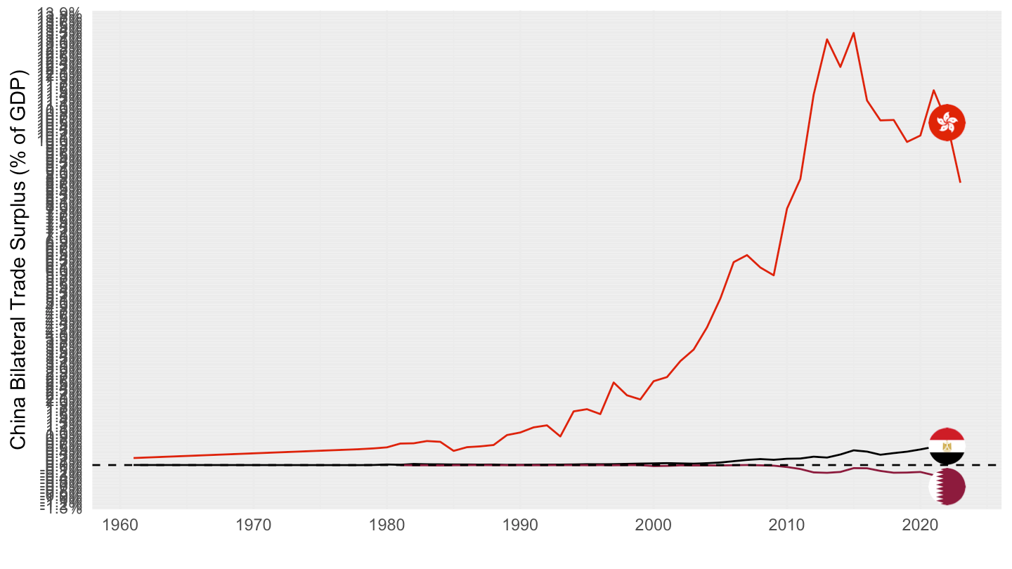
DOT_CN %>%
  filter(COUNTERPART_AREA  %in% c("DE", "NL", "BE"),
         INDICATOR %in% c("TBG_USD"),
         FREQ == "A") %>%
  inner_join(NGDP_USD %>%
              filter(REF_AREA == "FR",
                     FREQ == "A") %>%
              mutate(OBS_VALUE = OBS_VALUE*10^(UNIT_MULT)) %>%
              select(TIME_PERIOD, NGDP_USD = OBS_VALUE),
            by = "TIME_PERIOD") %>%
  year_to_date2 %>%
  mutate(OBS_VALUE = OBS_VALUE*10^(UNIT_MULT)/NGDP_USD) %>%
  left_join(COUNTERPART_AREA, by = "COUNTERPART_AREA") %>%
  mutate(Counterpart_area = ifelse(COUNTERPART_AREA == "U2", "Europe", Counterpart_area),
         Counterpart_area = ifelse(COUNTERPART_AREA == "W00", "World", Counterpart_area)) %>%
  left_join(colors, by = c("Counterpart_area" = "country")) %>%
  mutate(color = ifelse(COUNTERPART_AREA == "DE", color2, color)) %>%
  ggplot(.) + theme_minimal() + scale_color_identity() +
  geom_line(aes(x = date, y = OBS_VALUE, color = color)) +
  theme(legend.position = "none") + add_flags +
  scale_x_date(breaks = seq(1950, 2100, 10) %>% paste0("-01-01") %>% as.Date,
               labels = date_format("%Y")) +
  scale_y_continuous(breaks = 0.01*seq(-500, 500, .1),
                     labels = percent_format(accuracy = .1)) +
  xlab("") + ylab("China Bilateral Trade Surplus (% of GDP)") +
  geom_hline(yintercept = 0, linetype = "dashed", color = "black")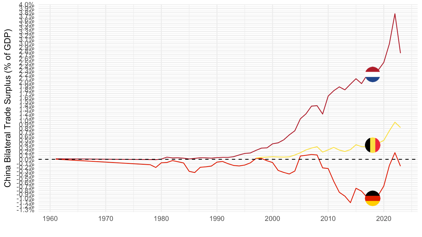
DOT_CN %>%
  filter(COUNTERPART_AREA  %in% c("DE", "NL", "BE", "W00"),
         INDICATOR %in% c("TBG_USD"),
         FREQ == "A") %>%
  inner_join(NGDP_USD %>%
              filter(REF_AREA == "FR",
                     FREQ == "A") %>%
              mutate(OBS_VALUE = OBS_VALUE*10^(UNIT_MULT)) %>%
              select(TIME_PERIOD, NGDP_USD = OBS_VALUE),
            by = "TIME_PERIOD") %>%
  year_to_date2 %>%
  mutate(OBS_VALUE = OBS_VALUE*10^(UNIT_MULT)/NGDP_USD) %>%
  left_join(COUNTERPART_AREA, by = "COUNTERPART_AREA") %>%
  mutate(Counterpart_area = ifelse(COUNTERPART_AREA == "U2", "Europe", Counterpart_area),
         Counterpart_area = ifelse(COUNTERPART_AREA == "W00", "World", Counterpart_area)) %>%
  left_join(colors, by = c("Counterpart_area" = "country")) %>%
  mutate(color = ifelse(COUNTERPART_AREA == "DE", color2, color)) %>%
  ggplot(.) + theme_minimal() + scale_color_identity() +
  geom_line(aes(x = date, y = OBS_VALUE, color = color)) +
  theme(legend.position = "none") + add_flags +
  scale_x_date(breaks = seq(1950, 2100, 10) %>% paste0("-01-01") %>% as.Date,
               labels = date_format("%Y")) +
  scale_y_continuous(breaks = 0.01*seq(-500, 500, .5),
                     labels = percent_format(accuracy = .1)) +
  xlab("") + ylab("China Bilateral Trade Surplus (% of GDP)") +
  geom_hline(yintercept = 0, linetype = "dashed", color = "black")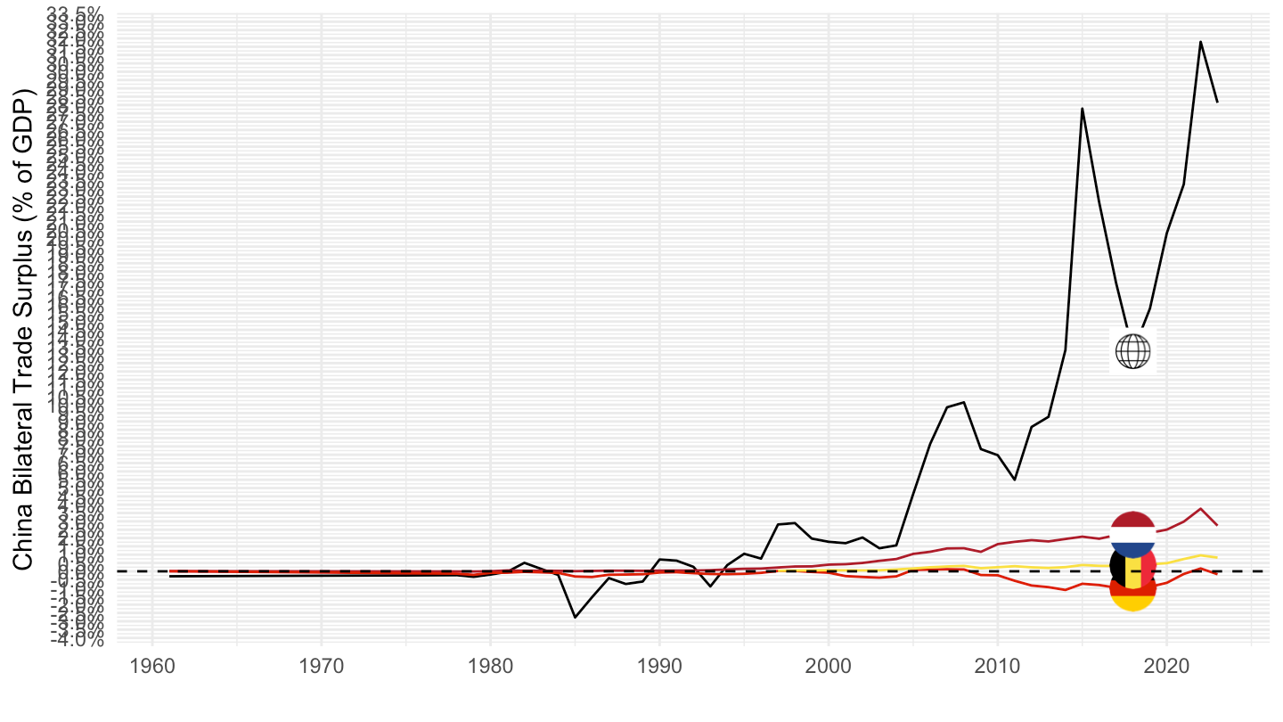
DOT_CN %>%
  filter(COUNTERPART_AREA  %in% c("DE", "NL", "BE", "W00"),
         INDICATOR %in% c("TBG_USD"),
         FREQ == "A") %>%
  inner_join(NGDP_USD %>%
              filter(REF_AREA == "FR",
                     FREQ == "A") %>%
              mutate(OBS_VALUE = OBS_VALUE*10^(UNIT_MULT)) %>%
              select(TIME_PERIOD, NGDP_USD = OBS_VALUE),
            by = "TIME_PERIOD") %>%
  year_to_date2 %>%
  filter(date >= as.Date("1990-01-01")) %>%
  mutate(OBS_VALUE = OBS_VALUE*10^(UNIT_MULT)/NGDP_USD) %>%
  left_join(COUNTERPART_AREA, by = "COUNTERPART_AREA") %>%
  mutate(Counterpart_area = ifelse(COUNTERPART_AREA == "U2", "Europe", Counterpart_area),
         Counterpart_area = ifelse(COUNTERPART_AREA == "W00", "World", Counterpart_area)) %>%
  left_join(colors, by = c("Counterpart_area" = "country")) %>%
  mutate(color = ifelse(COUNTERPART_AREA == "DE", color2, color)) %>%
  ggplot(.) + theme_minimal() + scale_color_identity() +
  geom_line(aes(x = date, y = OBS_VALUE, color = color)) +
  theme(legend.position = "none") + add_flags +
  scale_x_date(breaks = seq(1950, 2100, 5) %>% paste0("-01-01") %>% as.Date,
               labels = date_format("%Y")) +
  scale_y_continuous(breaks = 0.01*seq(-500, 500, .5),
                     labels = percent_format(accuracy = .1)) +
  xlab("") + ylab("China Bilateral Trade Surplus (% of GDP)") +
  geom_hline(yintercept = 0, linetype = "dashed", color = "black")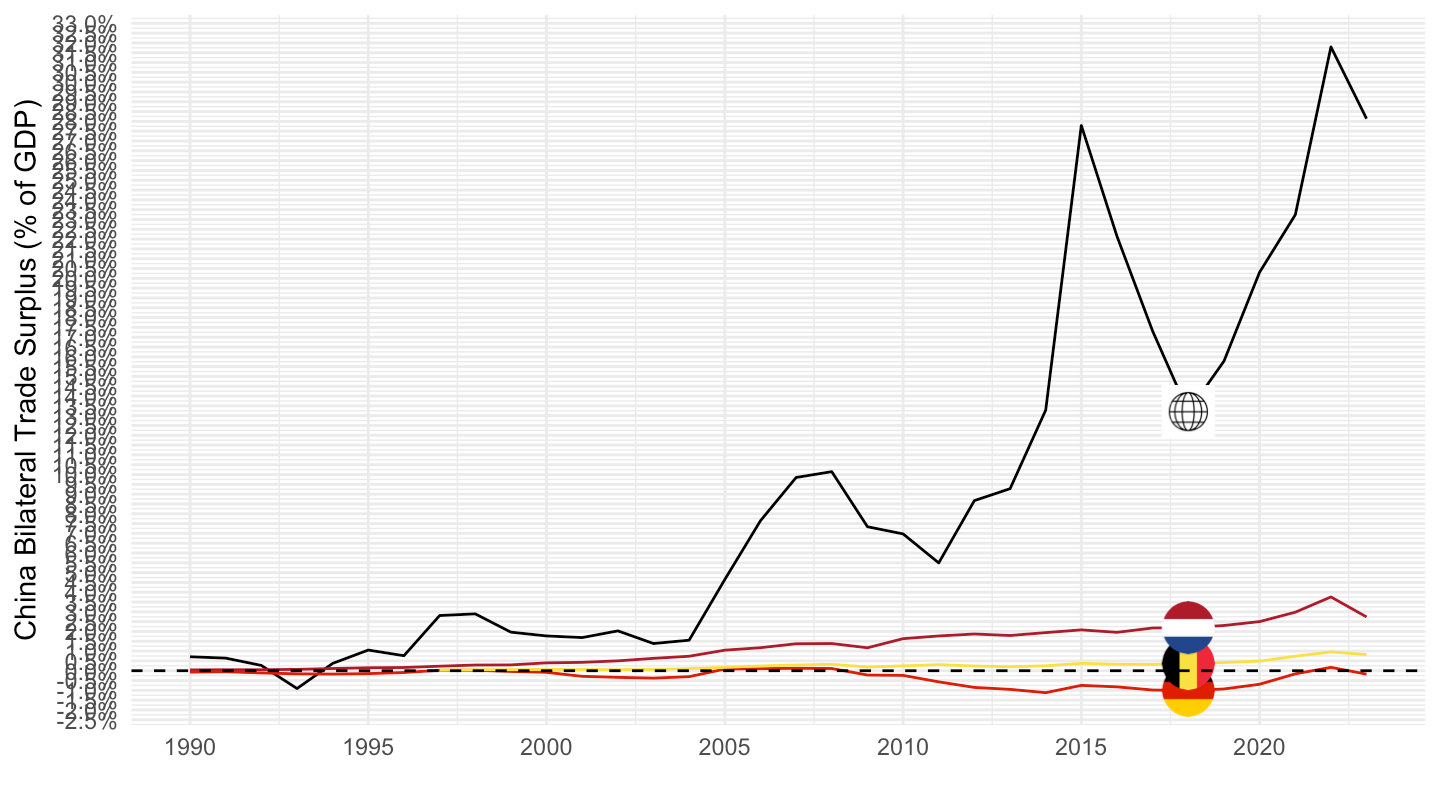
DOT_CN %>%
  filter(COUNTERPART_AREA  %in% c("CN", "IT", "ES"),
         INDICATOR %in% c("TBG_USD"),
         FREQ == "A") %>%
  inner_join(NGDP_USD %>%
              filter(REF_AREA == "FR",
                     FREQ == "A") %>%
              mutate(OBS_VALUE = OBS_VALUE*10^(UNIT_MULT)) %>%
              select(TIME_PERIOD, NGDP_USD = OBS_VALUE),
            by = "TIME_PERIOD") %>%
  year_to_date2 %>%
  mutate(OBS_VALUE = OBS_VALUE*10^(UNIT_MULT)/NGDP_USD) %>%
  left_join(COUNTERPART_AREA, by = "COUNTERPART_AREA") %>%
  mutate(Counterpart_area = ifelse(COUNTERPART_AREA == "U2", "Europe", Counterpart_area),
         Counterpart_area = ifelse(COUNTERPART_AREA == "W00", "World", Counterpart_area)) %>%
  left_join(colors, by = c("Counterpart_area" = "country")) %>%
  mutate(color = ifelse(COUNTERPART_AREA == "ES", color2, color)) %>%
  ggplot(.) + theme_minimal() + scale_color_identity() +
  geom_line(aes(x = date, y = OBS_VALUE, color = color)) +
  theme(legend.position = "none") + add_flags +
  scale_x_date(breaks = seq(1950, 2100, 10) %>% paste0("-01-01") %>% as.Date,
               labels = date_format("%Y")) +
  scale_y_continuous(breaks = 0.01*seq(-500, 500, .1),
                     labels = percent_format(accuracy = .1)) +
  xlab("") + ylab("China Bilateral Trade Surplus (% of GDP)") +
  geom_hline(yintercept = 0, linetype = "dashed", color = "black")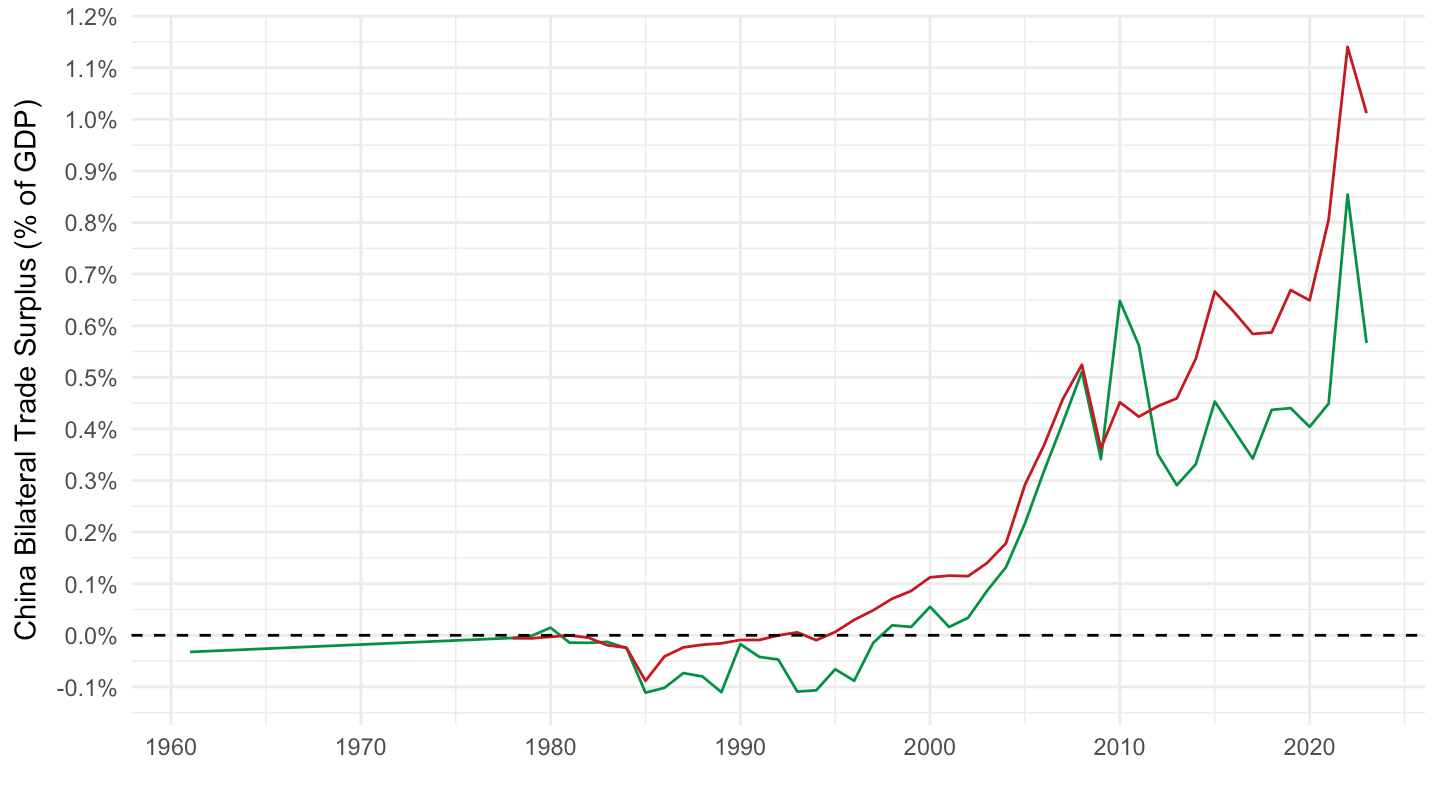
DOT_CN %>%
  filter(COUNTERPART_AREA  %in% c("CN", "DE", "U2"),
         INDICATOR %in% c("TBG_USD"),
         FREQ == "A") %>%
  inner_join(NGDP_USD %>%
              filter(REF_AREA == "FR",
                     FREQ == "A") %>%
              mutate(OBS_VALUE = OBS_VALUE*10^(UNIT_MULT)) %>%
              select(TIME_PERIOD, NGDP_USD = OBS_VALUE),
            by = "TIME_PERIOD") %>%
  year_to_date2 %>%
  mutate(OBS_VALUE = OBS_VALUE*10^(UNIT_MULT)/NGDP_USD) %>%
  left_join(COUNTERPART_AREA, by = "COUNTERPART_AREA") %>%
  mutate(Counterpart_area = ifelse(COUNTERPART_AREA == "U2", "Europe", Counterpart_area),
         Counterpart_area = ifelse(COUNTERPART_AREA == "W00", "World", Counterpart_area)) %>%
  left_join(colors, by = c("Counterpart_area" = "country")) %>%
  mutate(color = ifelse(COUNTERPART_AREA == "DE", color2, color)) %>%
  ggplot(.) + theme_minimal() + scale_color_identity() +
  geom_line(aes(x = date, y = OBS_VALUE, color = color)) +
  theme(legend.position = "none") + add_flags +
  scale_x_date(breaks = seq(1950, 2100, 10) %>% paste0("-01-01") %>% as.Date,
               labels = date_format("%Y")) +
  scale_y_continuous(breaks = 0.01*seq(-500, 500, 1),
                     labels = percent_format(accuracy = .1)) +
  xlab("") + ylab("China Bilateral Trade Surplus (% of GDP)") +
  geom_hline(yintercept = 0, linetype = "dashed", color = "black")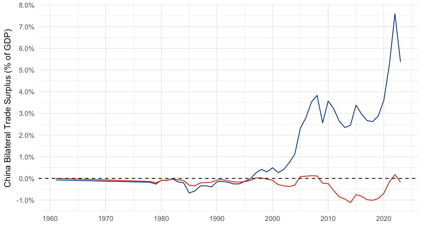
DOT_CN %>%
  filter(COUNTERPART_AREA  %in% c("CN", "DE", "U2"),
         INDICATOR %in% c("TBG_USD"),
         FREQ == "A") %>%
  inner_join(NGDP_USD %>%
              filter(REF_AREA == "FR",
                     FREQ == "A") %>%
              mutate(OBS_VALUE = OBS_VALUE*10^(UNIT_MULT)) %>%
              select(TIME_PERIOD, NGDP_USD = OBS_VALUE),
            by = "TIME_PERIOD") %>%
  year_to_date2 %>%
  filter(date >= as.Date("1980-01-01")) %>%
  mutate(OBS_VALUE = OBS_VALUE*10^(UNIT_MULT)/NGDP_USD) %>%
  left_join(COUNTERPART_AREA, by = "COUNTERPART_AREA") %>%
  mutate(Counterpart_area = ifelse(COUNTERPART_AREA == "U2", "Europe", Counterpart_area),
         Counterpart_area = ifelse(COUNTERPART_AREA == "W00", "World", Counterpart_area)) %>%
  left_join(colors, by = c("Counterpart_area" = "country")) %>%
  mutate(color = ifelse(COUNTERPART_AREA == "DE", color2, color)) %>%
  ggplot(.) + theme_minimal() + scale_color_identity() +
  geom_line(aes(x = date, y = OBS_VALUE, color = color)) +
  theme(legend.position = "none") + add_flags +
  scale_x_date(breaks = seq(1950, 2100, 10) %>% paste0("-01-01") %>% as.Date,
               labels = date_format("%Y")) +
  scale_y_continuous(breaks = 0.01*seq(-500, 500, 1),
                     labels = percent_format(accuracy = .1)) +
  xlab("") + ylab("China Bilateral Trade Surplus (% of GDP)") +
  geom_hline(yintercept = 0, linetype = "dashed", color = "black")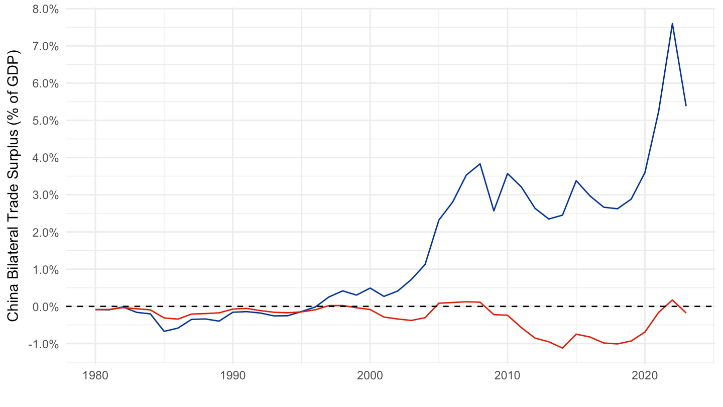
DOT_CN %>%
  filter(COUNTERPART_AREA  %in% c("CN", "DE", "U2"),
         INDICATOR %in% c("TBG_USD"),
         FREQ == "A") %>%
  inner_join(NGDP_USD %>%
              filter(REF_AREA == "FR",
                     FREQ == "A") %>%
              mutate(OBS_VALUE = OBS_VALUE*10^(UNIT_MULT)) %>%
              select(TIME_PERIOD, NGDP_USD = OBS_VALUE),
            by = "TIME_PERIOD") %>%
  year_to_date2 %>%
  filter(date >= as.Date("1990-01-01")) %>%
  mutate(OBS_VALUE = OBS_VALUE*10^(UNIT_MULT)/NGDP_USD) %>%
  left_join(COUNTERPART_AREA, by = "COUNTERPART_AREA") %>%
  mutate(Counterpart_area = ifelse(COUNTERPART_AREA == "U2", "Europe", Counterpart_area),
         Counterpart_area = ifelse(COUNTERPART_AREA == "W00", "World", Counterpart_area)) %>%
  left_join(colors, by = c("Counterpart_area" = "country")) %>%
  mutate(color = ifelse(COUNTERPART_AREA == "DE", color2, color)) %>%
  ggplot(.) + theme_minimal() + scale_color_identity() +
  geom_line(aes(x = date, y = OBS_VALUE, color = color)) +
  theme(legend.position = "none") + add_flags +
  scale_x_date(breaks = seq(1950, 2100, 10) %>% paste0("-01-01") %>% as.Date,
               labels = date_format("%Y")) +
  scale_y_continuous(breaks = 0.01*seq(-500, 500, 1),
                     labels = percent_format(accuracy = .1)) +
  xlab("") + ylab("China Bilateral Trade Surplus (% of GDP)") +
  geom_hline(yintercept = 0, linetype = "dashed", color = "black")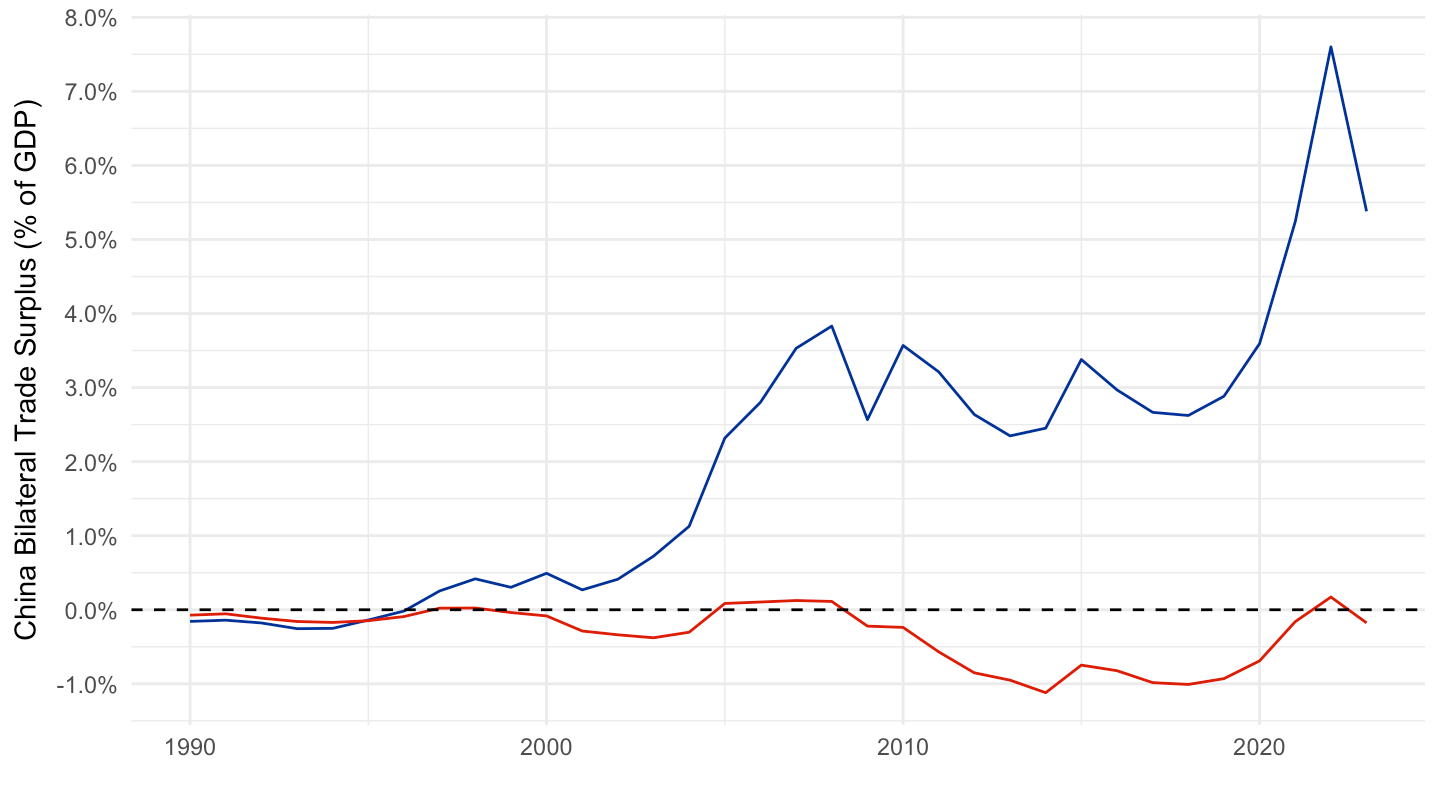
DOT_CN %>%
  filter(COUNTERPART_AREA  %in% c("CN", "DE", "U2", "RU"),
         INDICATOR %in% c("TBG_USD"),
         FREQ == "A") %>%
  inner_join(NGDP_USD %>%
              filter(REF_AREA == "FR",
                     FREQ == "A") %>%
              mutate(OBS_VALUE = OBS_VALUE*10^(UNIT_MULT)) %>%
              select(TIME_PERIOD, NGDP_USD = OBS_VALUE),
            by = "TIME_PERIOD") %>%
  year_to_date2 %>%
  mutate(OBS_VALUE = OBS_VALUE*10^(UNIT_MULT)/NGDP_USD) %>%
  left_join(COUNTERPART_AREA, by = "COUNTERPART_AREA") %>%
  mutate(Counterpart_area = ifelse(COUNTERPART_AREA == "U2", "Europe", Counterpart_area),
         Counterpart_area = ifelse(COUNTERPART_AREA == "W00", "World", Counterpart_area),
         Counterpart_area = ifelse(COUNTERPART_AREA == "RU", "Russia", Counterpart_area)) %>%
  left_join(colors, by = c("Counterpart_area" = "country")) %>%
  mutate(color = ifelse(COUNTERPART_AREA == "DE", color2, color)) %>%
  ggplot(.) + theme_minimal() + scale_color_identity() +
  geom_line(aes(x = date, y = OBS_VALUE, color = color)) +
  theme(legend.position = "none") + add_flags +
  scale_x_date(breaks = seq(1950, 2100, 10) %>% paste0("-01-01") %>% as.Date,
               labels = date_format("%Y")) +
  scale_y_continuous(breaks = 0.01*seq(-500, 500, 1),
                     labels = percent_format(accuracy = .1)) +
  xlab("") + ylab("China Bilateral Trade Surplus (% of GDP)") +
  geom_hline(yintercept = 0, linetype = "dashed", color = "black")