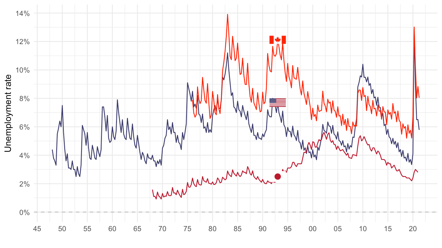
UNE_DEAP_SEX_AGE_RT_Q %>%
  filter(ref_area %in% c("USA", "JPN", "CAN"),
         sex == "SEX_T",
         classif1 == "AGE_AGGREGATE_TOTAL") %>%
  left_join(ref_area, by = "ref_area") %>%
  quarter_to_date() %>%
  left_join(colors, by = c("Ref_area" = "country")) %>%
  ggplot(.) + geom_line(aes(x = date, y = obs_value/100, color = color)) +
  geom_image(data = . %>%
               filter(date == as.Date("1993-01-01")) %>%
               mutate(image = paste0("../../icon/flag/", str_to_lower(gsub(" ", "-", Ref_area)), ".png")),
             aes(x = date, y = obs_value/100, image = image), asp = 1.5) +
  scale_color_identity() + theme_minimal() +
  xlab("") + ylab("Unemployment rate") +
  theme(legend.title = element_blank(),
        legend.position = c(0.15, 0.85)) +
  scale_x_date(breaks = seq(1900, 2020, 5) %>% paste0("-01-01") %>% as.Date,
               labels = date_format("%y")) +
  scale_y_continuous(breaks = 0.01*seq(-100, 10000, 2),
                     labels = percent_format(a = 1)) +
  geom_hline(yintercept = 0, linetype = "dashed", color = "grey")