
Last observation: 2020 (N = 265)
First observation: 1991 (N = 265)
Last data update: 01 août 2026, 21:27
Last compile: 25 oct. 2026, 22:44
EMP_2IND_NOC_RT_A |>
  left_join(source, by = "source") |>
  group_by(source, Source) |>
  summarise(Nobs = n()) |>
  arrange(-Nobs) %>%
{if (is_html_output()) datatable(., filter = 'top', rownames = F) else .}EMP_2IND_NOC_RT_A |>
left_join(ref_area, by = "ref_area") |>
group_by(ref_area, Ref_area) |>
summarise(Nobs = n()) |>
arrange(-Nobs) |>
mutate(Flag = gsub(" ", "-", str_to_lower(Ref_area)),
Flag = paste0('<img src="../../bib/flags/vsmall/', Flag, '.png" alt="Flag">')) |>
select(Flag, everything()) %>%
{if (is_html_output()) datatable(., filter = 'top', rownames = F, escape = F) else .}EMP_2IND_NOC_RT_A |>
year_to_date() |>
filter(ref_area %in% c("DEU", "FRA", "USA", "CHE")) |>
left_join(ref_area, by = "ref_area") |>
mutate(obs_value = obs_value/100) |>
add_flag_color("Ref_area") |>
ggplot() + scale_color_identity() + add_flags + theme_minimal() +
geom_line(aes(x = date, y = obs_value, color = color)) +
scale_x_date(breaks = seq(1920, 2100, 2) |> paste0("-01-01") |> as.Date(),
labels = date_format("%Y")) +
theme(legend.position = c(0.85, 0.8),
legend.title = element_blank()) +
scale_y_continuous(breaks = 0.01*seq(0, 90, 2),
labels = percent_format(accuracy = 1)) +
ylab("Industry (% of total employment)") + xlab("")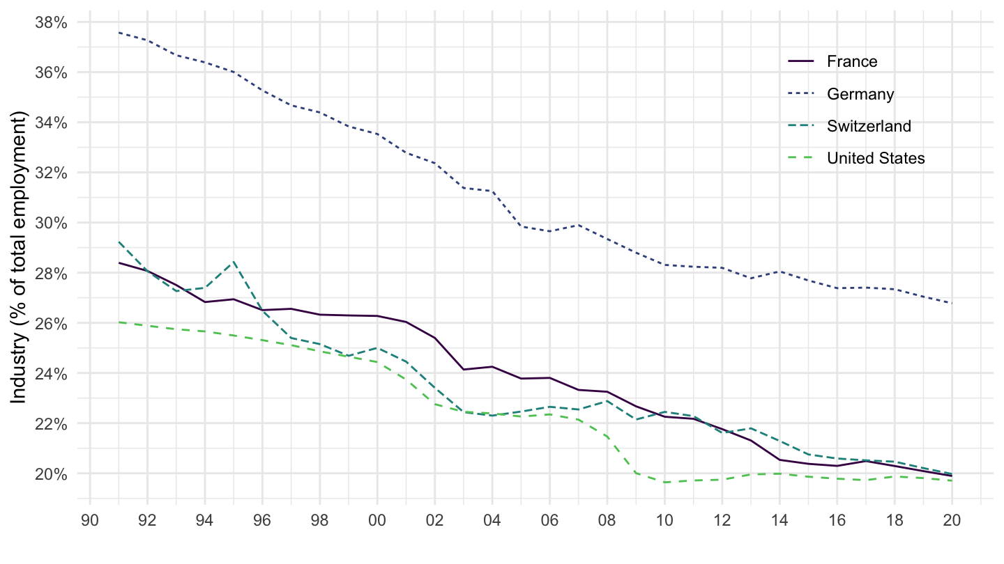
EMP_2IND_NOC_RT_A |>
  year_to_date() |>
  filter(ref_area %in% c("SWE", "GBR", "ESP", "ITA")) |>
  left_join(ref_area, by = "ref_area") |>
  mutate(obs_value = obs_value/100) |>
  add_flag_color("Ref_area") |>
  ggplot() + scale_color_identity() + add_flags + theme_minimal() +
  geom_line(aes(x = date, y = obs_value, color = color)) +
  scale_x_date(breaks = seq(1920, 2100, 2) |> paste0("-01-01") |> as.Date(),
               labels = date_format("%Y")) +
  theme(legend.position = c(0.85, 0.8),
        legend.title = element_blank()) +
  scale_y_continuous(breaks = 0.01*seq(0, 90, 2),
                     labels = percent_format(accuracy = 1)) +
  ylab("Industry (% of total employment)") + xlab("")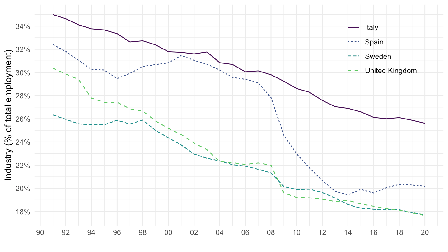
| source | dataset | Title | Updated |
|---|---|---|---|


