Table B.101 Balance Sheet of Households and Nonprofit Organizations - B101
Data - FRB
Layout
png
Javascript
Code
Z1_csv_var %>%
  filter(table == "B101") %>%
  select(pos, variable, variable_desc) %>%
  print_table_conditional()
Checkable Deposits
All
Code
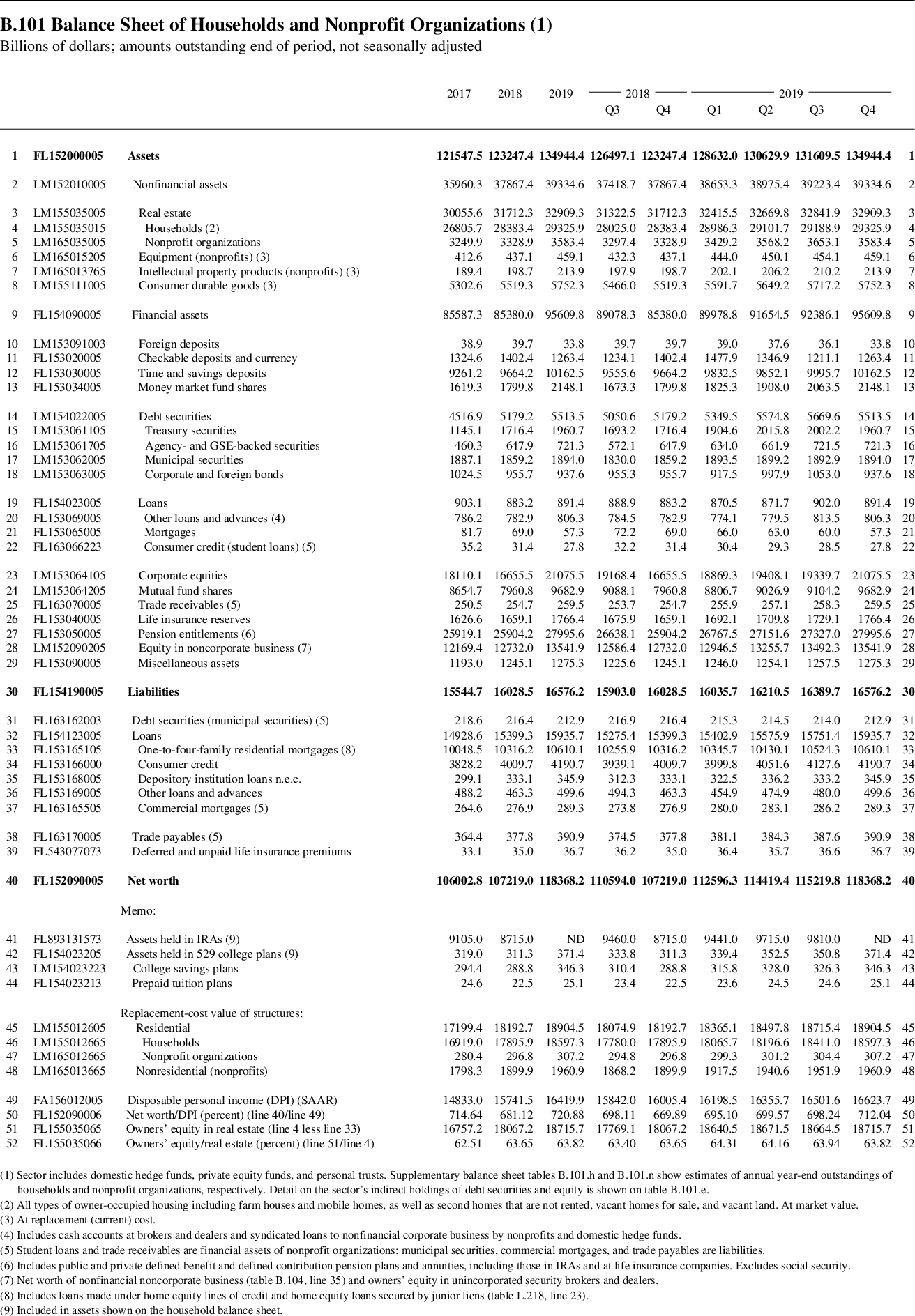
Z1 %>%
  filter(SERIES_NAME %in% c("FL153020005.Q", "FA086902005.Q"),
         OBS_STATUS == "A") %>%
  select(SERIES_NAME, TIME_PERIOD, OBS_VALUE) %>%
  spread(SERIES_NAME, OBS_VALUE) %>%
  ggplot(.) + theme_minimal() +
  geom_line(aes(x = TIME_PERIOD, y = `FL153020005.Q`/`FA086902005.Q`)) +
  theme(legend.title = element_blank(),
        legend.position = c(0.4, 0.9)) +
  scale_x_date(breaks = seq(1930, 2100, 5) %>% paste0("-01-01") %>% as.Date,
               labels = date_format("%Y")) +
  ylab("HH checkable deposits and currency (% of GDP)") + xlab("") +
  geom_rect(data = nber_recessions %>%
              filter(Peak > as.Date("1950-01-01")),
            aes(xmin = Peak, xmax = Trough, ymin = -Inf, ymax = +Inf),
            fill = 'grey', alpha = 0.5) +

  scale_y_continuous(breaks = 0.01*seq(-100, 600, 2),
                     labels = scales::percent_format(accuracy = 1))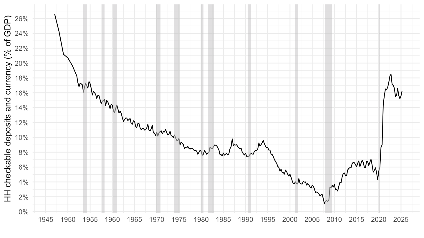
1990-
Code
Z1 %>%
  filter(SERIES_NAME %in% c("FL153020005.Q", "FA086902005.Q"),
         OBS_STATUS == "A",
         TIME_PERIOD >= as.Date("2000-01-01")) %>%
  select(SERIES_NAME, TIME_PERIOD, OBS_VALUE) %>%
  spread(SERIES_NAME, OBS_VALUE) %>%
  ggplot(.) + theme_minimal() +
  geom_line(aes(x = TIME_PERIOD, y = `FL153020005.Q`/`FA086902005.Q`)) +
  theme(legend.title = element_blank(),
        legend.position = c(0.4, 0.9)) +
  scale_x_date(breaks = seq(1930, 2100, 5) %>% paste0("-01-01") %>% as.Date,
               labels = date_format("%Y")) +
  ylab("HH checkable deposits and currency (% of GDP)") + xlab("") +
  geom_rect(data = nber_recessions %>%
              filter(Peak > as.Date("2000-01-01")),
            aes(xmin = Peak, xmax = Trough, ymin = -Inf, ymax = +Inf),
            fill = 'grey', alpha = 0.5) +

  scale_y_continuous(breaks = 0.01*seq(-100, 600, 2),
                     labels = scales::percent_format(accuracy = 1))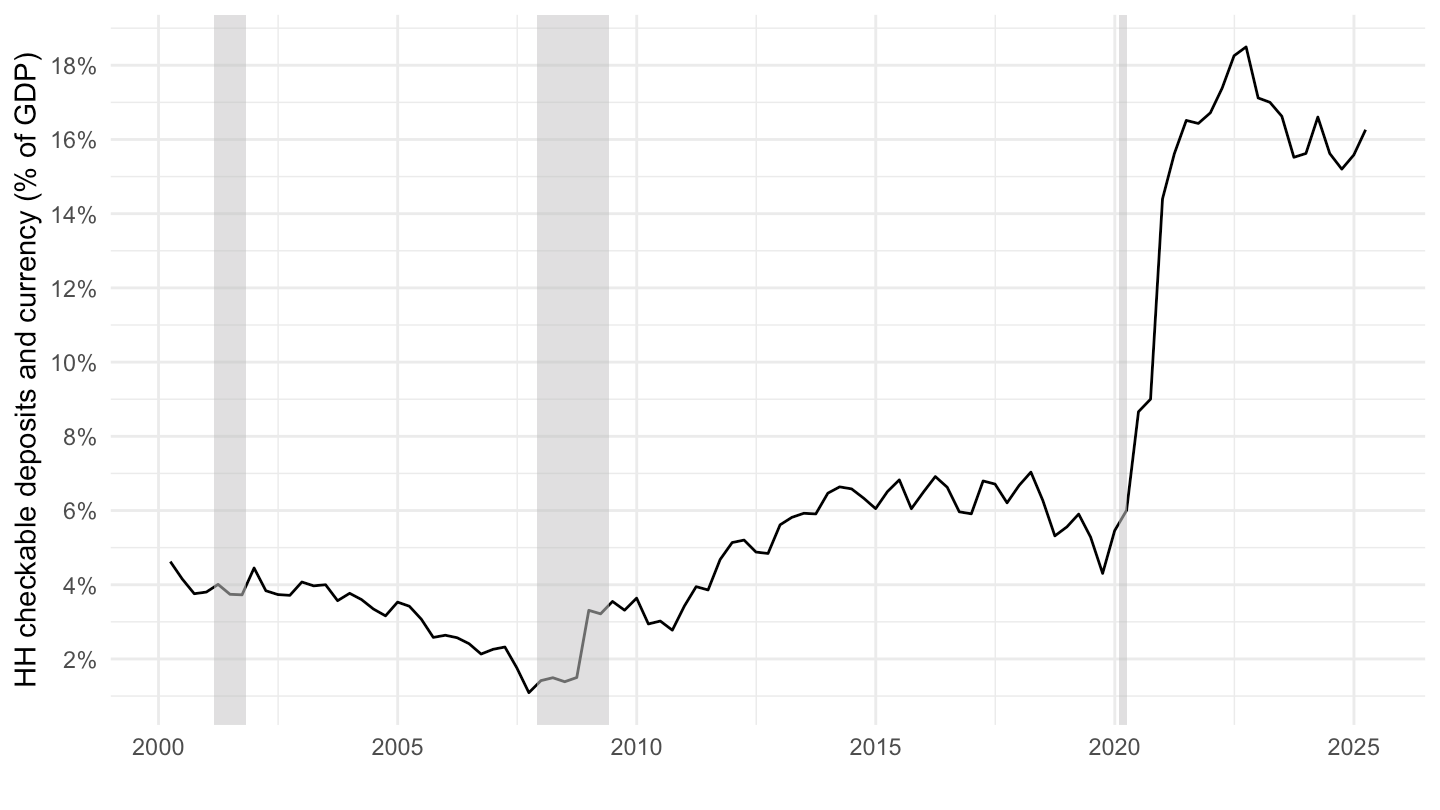
1990-
Code
Z1 %>%
  filter(SERIES_NAME %in% c("FL153020005.Q", "FA086902005.Q", "LM713061103.Q"),
         OBS_STATUS == "A",
         TIME_PERIOD >= as.Date("2000-01-01")) %>%
  select(SERIES_NAME, TIME_PERIOD, OBS_VALUE) %>%
  spread(SERIES_NAME, OBS_VALUE) %>%
  transmute(TIME_PERIOD,
            `Checkable deposits and currency held by Households` = `FL153020005.Q`/`FA086902005.Q`,
            `Treasury securities held by the Central Bank` = `LM713061103.Q`/`FA086902005.Q`) %>%
  gather(variable, value, -TIME_PERIOD) %>%
  ggplot(.) + theme_minimal() +
  geom_line(aes(x = TIME_PERIOD, y = value, color = variable)) +
  theme(legend.title = element_blank(),
        legend.position = c(0.4, 0.9)) +
  scale_x_date(breaks = seq(1930, 2100, 5) %>% paste0("-01-01") %>% as.Date,
               labels = date_format("%Y")) +
  ylab("% of GDP") + xlab("") +
  geom_rect(data = nber_recessions %>%
              filter(Peak > as.Date("2000-01-01")),
            aes(xmin = Peak, xmax = Trough, ymin = -Inf, ymax = +Inf),
            fill = 'grey', alpha = 0.5) +
  scale_color_manual(values = viridis(3)[1:2]) +
  scale_y_continuous(breaks = 0.01*seq(-100, 600, 2),
                     labels = scales::percent_format(accuracy = 1))
Liabilities
Code
Z1_csv_var %>%
  mutate(line = parse_number(pos)) %>%
  filter(table == "B101",
         line %in% c(30, 33, 34)) %>%
  left_join(Z1_csv, by = c("variable", "table")) %>%
  select(date, table, pos, variable_desc, value) %>%
  left_join(gdp_Q %>% rename(gdp = value), by = "date") %>%
  mutate(value = value / gdp) %>%
  ggplot(.) + theme_minimal() +
  geom_line(aes(x = date, y = value, color = variable_desc)) +
  theme(legend.title = element_blank(),
        legend.position = c(0.4, 0.9)) +
  scale_x_date(breaks = seq(1930, 2100, 5) %>% paste0("-01-01") %>% as.Date,
               labels = date_format("%Y")) +
  ylab("% of GDP") + xlab("") +
  geom_rect(data = nber_recessions %>%
              filter(Peak > as.Date("1950-01-01")),
            aes(xmin = Peak, xmax = Trough, ymin = -Inf, ymax = +Inf),
            fill = 'grey', alpha = 0.5) +

  scale_y_continuous(breaks = 0.01*seq(-100, 600, 10),
                     labels = scales::percent_format(accuracy = 1))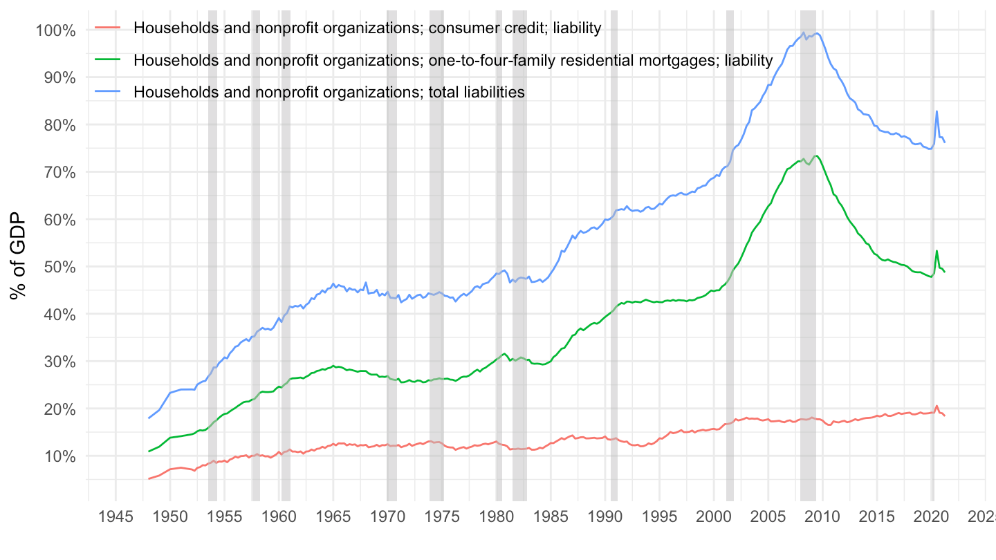
Structures, Real Estate
Code
Z1_csv_var %>%
  mutate(line = parse_number(pos)) %>%
  filter(table == "B101",
         line %in% c(4, 46)) %>%
  left_join(Z1_csv, by = c("variable", "table")) %>%
  select(date, table, pos, variable_desc, value) %>%
  left_join(gdp_Q %>% rename(gdp = value), by = "date") %>%
  mutate(value = value / gdp) %>%
  ggplot(.) + theme_minimal() +
  geom_line(aes(x = date, y = value, color = variable_desc)) +
  theme(legend.title = element_blank(),
        legend.position = c(0.5, 0.9)) +
  scale_x_date(breaks = seq(1930, 2100, 5) %>% paste0("-01-01") %>% as.Date,
               labels = date_format("%Y")) +
  ylab("% of GDP") + xlab("") +
  geom_rect(data = nber_recessions %>%
              filter(Peak > as.Date("1950-01-01")),
            aes(xmin = Peak, xmax = Trough, ymin = -Inf, ymax = +Inf),
            fill = 'grey', alpha = 0.5) +

  scale_y_continuous(breaks = 0.01*seq(-100, 600, 10),
                     labels = scales::percent_format(accuracy = 1),
                     limits = c(0.5, 2))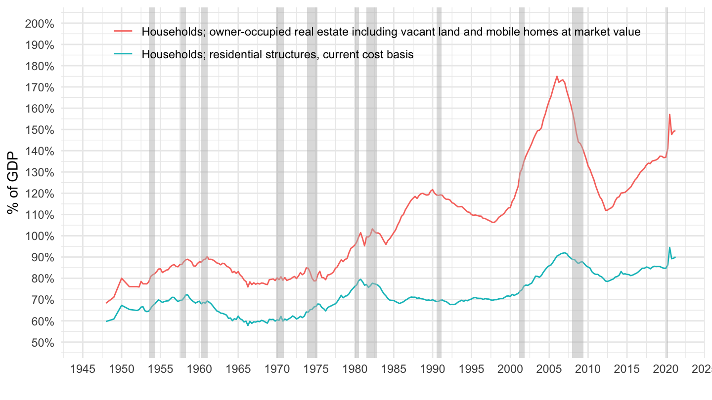
Net Worth
Code
Z1_csv_var %>%
  mutate(line = parse_number(pos)) %>%
  filter(table == "B101",
         line %in% c(1, 9, 40)) %>%
  left_join(Z1_csv, by = c("variable", "table")) %>%
  select(date, table, pos, variable_desc, value) %>%
  left_join(gdp_Q %>% rename(gdp = value), by = "date") %>%
  mutate(value = value / gdp) %>%
  ggplot(.) + theme_minimal() +
  geom_line(aes(x = date, y = value, color = variable_desc)) +
  theme(legend.title = element_blank(),
        legend.position = c(0.4, 0.9)) +
  scale_x_date(breaks = seq(1930, 2100, 5) %>% paste0("-01-01") %>% as.Date,
               labels = date_format("%Y")) +
  ylab("% of GDP") + xlab("") +
  geom_rect(data = nber_recessions %>%
              filter(Peak > as.Date("1950-01-01")),
            aes(xmin = Peak, xmax = Trough, ymin = -Inf, ymax = +Inf),
            fill = 'grey', alpha = 0.5) +

  scale_y_continuous(breaks = 0.01*seq(-100, 700, 50),
                     labels = scales::percent_format(accuracy = 1))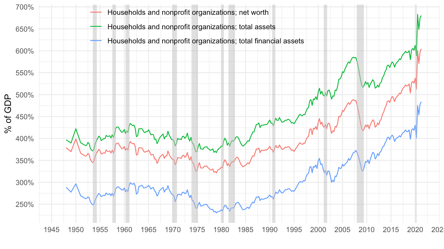
Corporate Equities, Pensions, Real Estate
Code
Z1_csv_var %>%
  mutate(line = parse_number(pos)) %>%
  filter(table == "B101",
         line %in% c(23, 27, 3)) %>%
  left_join(Z1_csv, by = c("variable", "table")) %>%
  select(date, table, pos, variable_desc, value) %>%
  left_join(gdp_Q %>% rename(gdp = value), by = "date") %>%
  mutate(value = value / gdp) %>%
  ggplot(.) + theme_minimal() +
  geom_line(aes(x = date, y = value, color = variable_desc)) +
  theme(legend.title = element_blank(),
        legend.position = c(0.4, 0.9)) +
  scale_x_date(breaks = seq(1930, 2100, 5) %>% paste0("-01-01") %>% as.Date,
               labels = date_format("%Y")) +
  ylab("% of GDP") + xlab("") +
  geom_rect(data = nber_recessions %>%
              filter(Peak > as.Date("1950-01-01")),
            aes(xmin = Peak, xmax = Trough, ymin = -Inf, ymax = +Inf),
            fill = 'grey', alpha = 0.5) +

  scale_y_continuous(breaks = 0.01*seq(-100, 600, 10),
                     labels = scales::percent_format(accuracy = 1))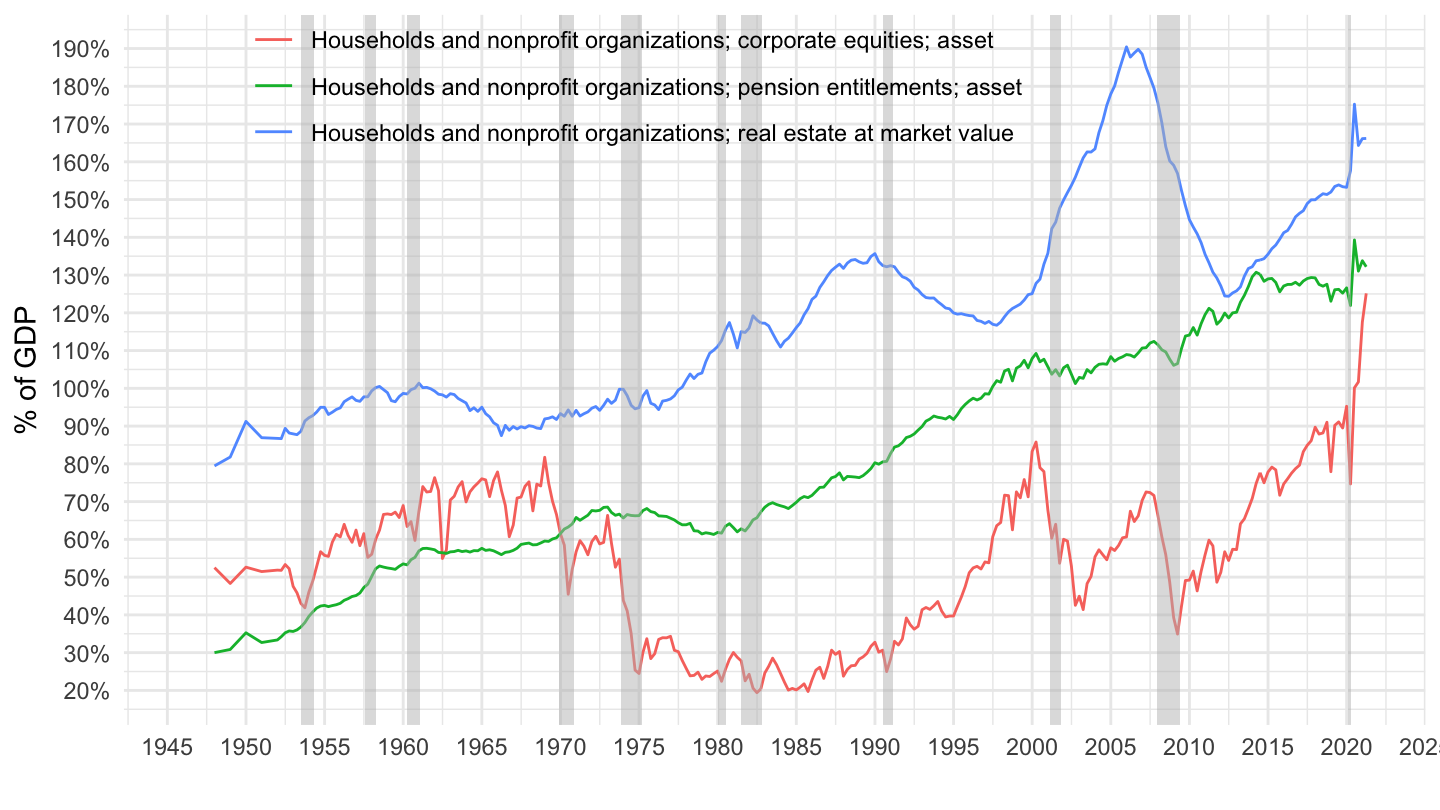
Residential Structures
Code
Z1_csv_var %>%
  mutate(line = parse_number(pos)) %>%
  filter(table == "B101",
         line %in% c(45, 46)) %>%
  left_join(Z1_csv, by = c("variable", "table")) %>%
  select(date, table, pos, variable_desc, value) %>%
  left_join(gdp_Q %>% rename(gdp = value), by = "date") %>%
  mutate(value = value / gdp) %>%
  ggplot(.) + theme_minimal() +
  geom_line(aes(x = date, y = value, color = variable_desc)) +
  theme(legend.title = element_blank(),
        legend.position = c(0.4, 0.9)) +
  scale_x_date(breaks = seq(1930, 2100, 5) %>% paste0("-01-01") %>% as.Date,
               labels = date_format("%Y")) +
  ylab("% of GDP") + xlab("") +
  geom_rect(data = nber_recessions %>%
              filter(Peak > as.Date("1950-01-01")),
            aes(xmin = Peak, xmax = Trough, ymin = -Inf, ymax = +Inf),
            fill = 'grey', alpha = 0.5) +

  scale_y_continuous(breaks = 0.01*seq(-100, 600, 10),
                     labels = scales::percent_format(accuracy = 1))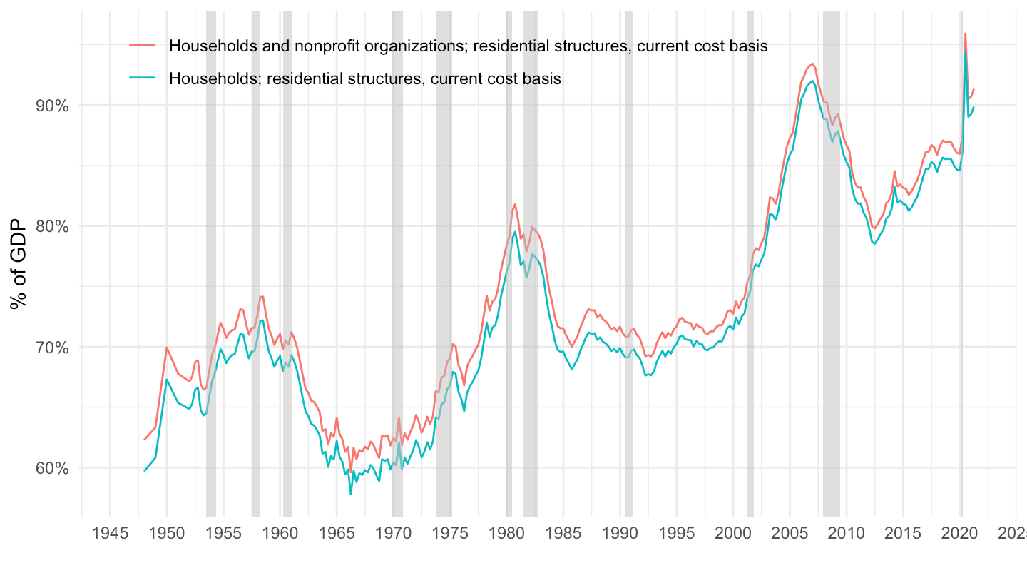
2019
Billions
Code
Z1_csv_var %>%
  filter(table == "B101") %>%
  left_join(Z1_csv %>%
              filter(date == as.Date("2019-12-31")),
            by = c("variable", "table")) %>%
  select(table, pos, variable_desc, value) %>%
  mutate(value = round(value/1000) %>% paste0("$ ", ., " Bn")) %>%
  {if (is_html_output()) datatable(., filter = 'top', rownames = F) else .}