Table B.1 Derivation of U.S. Net Wealth - B1
Data - FRB
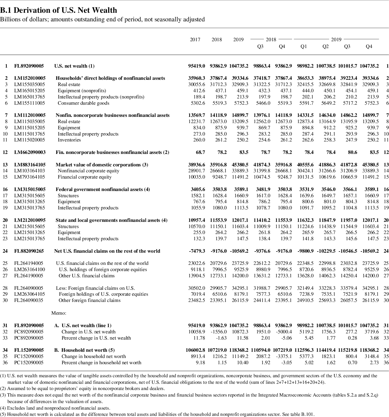
Example: LM152010005.Q
LM152010005.Q: Households and nonprofit organizations; nonfinancial assets
– SERIES_PREFIX == “LM”: Market value levels, NSA
– SERIES_SECTOR == “15”: Households and nonprofit organizations (S14+S15)
– SERIES_INSTRUMENT == “20100”: Nonfinancial assets
– SERIES_TYPE == “5”: Computed series
Layout
Examples
Net Worth
Z1_csv
All
Code
Z1_table_variable %>%
  mutate(line = parse_number(pos)) %>%
  filter(table == "B1",
         line %in% c(2, 7, 13)) %>%
  left_join(Z1_csv, by = c("variable", "table")) %>%
  select(date, table, pos, Variable, value) %>%
  left_join(gdp_Q %>% rename(gdp = value), by = "date") %>%
  mutate(value = value / gdp) %>%
  ggplot(.) + theme_minimal() +
  geom_line(aes(x = date, y = value, color = Variable, linetype = Variable)) +
  theme(legend.title = element_blank(),
        legend.position = c(0.4, 0.9)) +
  scale_x_date(breaks = seq(1930, 2100, 5) %>% paste0("-01-01") %>% as.Date,
               labels = date_format("%Y")) +
  ylab("% of GDP") + xlab("") +
  geom_rect(data = nber_recessions %>%
              filter(Peak > as.Date("1950-01-01")),
            aes(xmin = Peak, xmax = Trough, ymin = -Inf, ymax = +Inf),
            fill = 'grey', alpha = 0.5) +
  scale_color_manual(values = viridis(4)[1:3]) +
  scale_y_continuous(breaks = 0.01*seq(-100, 700, 50),
                     labels = scales::percent_format(accuracy = 1))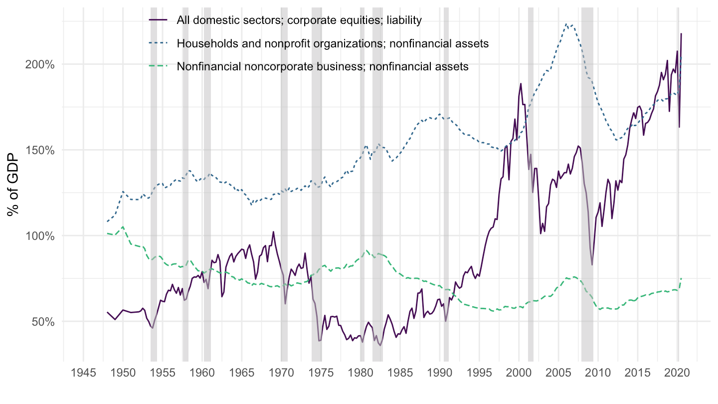
2000-
Code
Z1_table_variable %>%
  mutate(line = parse_number(pos)) %>%
  filter(table == "B1",
         line %in% c(2, 7, 13)) %>%
  left_join(Z1_csv, by = c("variable", "table")) %>%
  select(date, table, pos, Variable, value) %>%
  left_join(gdp_Q %>% rename(gdp = value), by = "date") %>%
  mutate(value = value / gdp) %>%
  filter(date >= as.Date("2000-01-01")) %>%
  ggplot(.) + theme_minimal() +
  geom_line(aes(x = date, y = value, color = Variable, linetype = Variable)) +
  theme(legend.title = element_blank(),
        legend.position = c(0.4, 0.9)) +
  scale_x_date(breaks = seq(1930, 2100, 5) %>% paste0("-01-01") %>% as.Date,
               labels = date_format("%Y")) +
  ylab("% of GDP") + xlab("") +
  geom_rect(data = nber_recessions %>%
              filter(Peak > as.Date("2000-01-01")),
            aes(xmin = Peak, xmax = Trough, ymin = -Inf, ymax = +Inf),
            fill = 'grey', alpha = 0.5) +
  scale_color_manual(values = viridis(4)[1:3]) +
  scale_y_continuous(breaks = 0.01*seq(-100, 700, 50),
                     labels = scales::percent_format(accuracy = 1))
Z1_SDMX
Code
Z1 %>%
  filter(SERIES_NAME %in% c("LM152010005.Q", "LM112010005.Q", "LM883164105.Q"),
         OBS_STATUS != "ND") %>%
  rename(date = TIME_PERIOD) %>%
  left_join(gdp_Q %>%
              rename(gdp = value), by = "date") %>%
  left_join(SERIES_SECTOR, by = "SERIES_SECTOR") %>%
  left_join(SERIES_INSTRUMENT, by = "SERIES_INSTRUMENT") %>%
  ggplot(.) + theme_minimal() + ylab("% of GDP") + xlab("") +
  geom_line(aes(x = date, y = OBS_VALUE / gdp, color = paste0(Series_instrument, Series_sector))) +
  theme(legend.title = element_blank(),
        legend.position = c(0.4, 0.8)) +
  scale_x_date(breaks = seq(1930, 2100, 5) %>% paste0("-01-01") %>% as.Date,
               labels = date_format("%Y")) +
  geom_rect(data = nber_recessions %>%
              filter(Peak > as.Date("1950-01-01")),
            aes(xmin = Peak, xmax = Trough, ymin = -Inf, ymax = +Inf),
            fill = 'grey', alpha = 0.5) +
  scale_color_manual(values = viridis(4)[1:3]) +
  scale_y_continuous(breaks = 0.01*seq(-100, 700, 50),
                     labels = scales::percent_format(accuracy = 1))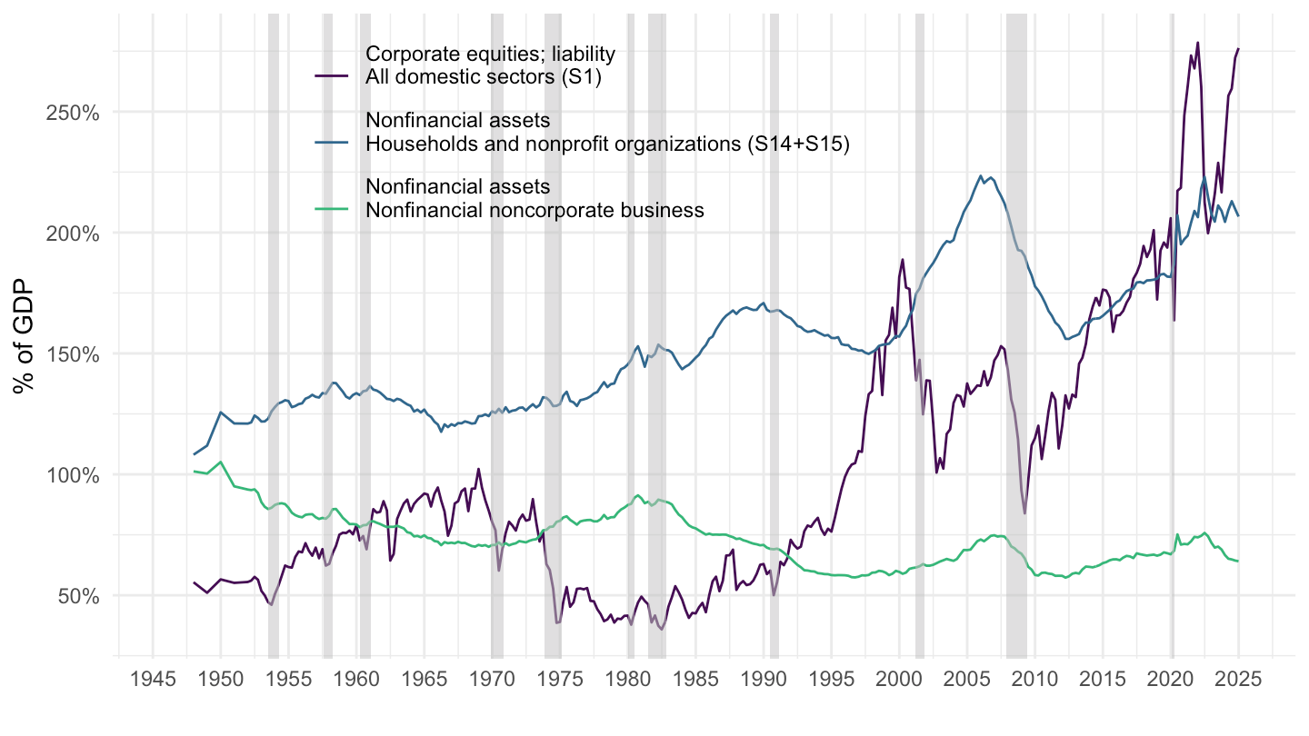
Corporate Equities, Pensions, Real Estate
Code
Z1_table_variable %>%
  mutate(line = parse_number(pos)) %>%
  filter(table == "B1",
         line %in% c(31,34)) %>%
  left_join(Z1_csv, by = c("variable", "table")) %>%
  select(date, table, pos, Variable, value) %>%
  left_join(gdp_Q %>% rename(gdp = value), by = "date") %>%
  mutate(value = value / gdp) %>%
  ggplot(.) + theme_minimal() + ylab("% of GDP") + xlab("") +
  geom_line(aes(x = date, y = value, color = Variable)) +
  theme(legend.title = element_blank(),
        legend.position = c(0.4, 0.9)) +
  scale_x_date(breaks = seq(1930, 2100, 5) %>% paste0("-01-01") %>% as.Date,
               labels = date_format("%Y")) +
  geom_rect(data = nber_recessions %>%
              filter(Peak > as.Date("1950-01-01")),
            aes(xmin = Peak, xmax = Trough, ymin = -Inf, ymax = +Inf),
            fill = 'grey', alpha = 0.5) +
  scale_color_manual(values = viridis(3)[1:2]) +
  scale_y_continuous(breaks = 0.01*seq(-100, 600, 20),
                     labels = scales::percent_format(accuracy = 1))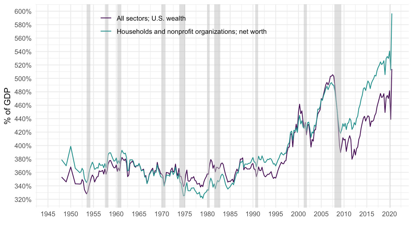
Corporate Equities, Real Estate
English
Code
Z1_table_variable %>%
  mutate(line = parse_number(pos)) %>%
  filter(table == "B1",
         line %in% c(3, 14)) %>%
  left_join(Z1_csv, by = c("variable", "table")) %>%
  left_join(gdp_Q %>% rename(gdp = value), by = "date") %>%
  mutate(value = value / gdp,
         Variable = case_when(line == 3 ~ "Real estate (households)",
                              line == 14 ~ "Equities (corporate sector)")) %>%
  ggplot(.) + theme_minimal() +
  geom_line(aes(x = date, y = value, color = Variable, linetype = Variable)) +
  theme(legend.title = element_blank(),
        legend.position = c(0.4, 0.9)) +
  scale_x_date(breaks = seq(1930, 2100, 5) %>% paste0("-01-01") %>% as.Date,
               labels = date_format("%Y")) +
  ylab("% of GDP") + xlab("") +
  geom_rect(data = nber_recessions %>%
              filter(Peak > as.Date("1950-01-01")),
            aes(xmin = Peak, xmax = Trough, ymin = -Inf, ymax = +Inf),
            fill = 'grey', alpha = 0.5) +
  scale_color_manual(values = viridis(4)[1:3]) +
  scale_y_continuous(breaks = 0.01*seq(-100, 600, 10),
                     labels = scales::percent_format(accuracy = 1))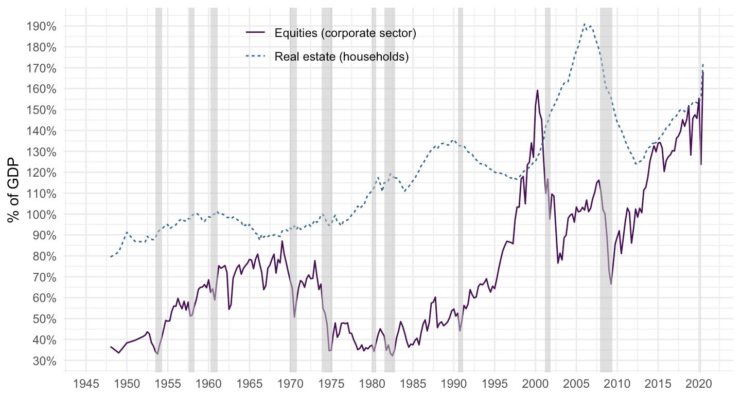
Français
Code
Z1_table_variable %>%
  mutate(line = parse_number(pos)) %>%
  filter(table == "B1",
         line %in% c(3, 14)) %>%
  left_join(Z1_csv, by = c("variable", "table")) %>%
  left_join(gdp_Q %>% rename(gdp = value), by = "date") %>%
  mutate(value = value / gdp,
         Variable = case_when(line == 3 ~ "Immobilier (ménages)",
                              line == 14 ~ "Actions (secteur corporate)")) %>%
  ggplot(.) + theme_minimal() +
  geom_line(aes(x = date, y = value, color = Variable)) +
  theme(legend.title = element_blank(),
        legend.position = c(0.4, 0.9)) +
  scale_x_date(breaks = seq(1930, 2100, 5) %>% paste0("-01-01") %>% as.Date,
               labels = date_format("%Y")) +
  ylab("% du PIB ") + xlab("") +
  geom_rect(data = nber_recessions %>%
              filter(Peak > as.Date("1950-01-01")),
            aes(xmin = Peak, xmax = Trough, ymin = -Inf, ymax = +Inf),
            fill = 'grey', alpha = 0.5) +
  scale_color_manual(values = viridis(3)[1:2]) +
  scale_y_continuous(breaks = 0.01*seq(-100, 600, 10),
                     labels = scales::percent_format(accuracy = 1))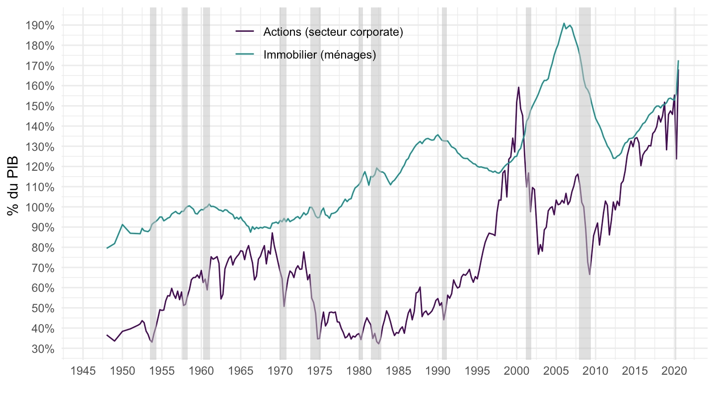
2019
Billions
Code
Z1_table_variable %>%
  filter(table == "B1") %>%
  left_join(Z1_csv %>%
              filter(date == as.Date("2019-12-31")),
            by = c("variable", "table")) %>%
  select(table, pos, Variable, value) %>%
  mutate(value = round(value/1000) %>% paste0("$ ", ., " Bn")) %>%
  {if (is_html_output()) datatable(., filter = 'top', rownames = F) else .}