Youth unemployment rate by sex, age and NUTS 2 regions - yth_empl_110

Data - Eurostat

Author

François Geerolf

Info

Last observation: Annual: 2025 (N = 7,830)

First observation: Annual: 1999 (N = 6,786)

Last data update: 23 jul 2026, 22:30. Last compile: 24 jul 2026, 04:10

Structure

2018 Map

Code

europe_NUTS0_new <- yth_empl_110 %>%
  filter(sex == "T",
         time == "2018") %>%
  select(geo, values) %>%
  right_join(europe_NUTS0 %>%
               filter(long >= -10,
                      lat >= 20), by = "geo") %>%
  group_by(geo, values) %>%
  summarise(long = mean(long), lat = mean(lat))

yth_empl_110 %>%
  filter(sex == "T",
         time == "2018") %>%
  select(geo, values) %>%
  right_join(europe_NUTS0 %>%
               filter(long >= -10,
                      lat >= 20), by = "geo") %>%
  ggplot(aes(x = long, y = lat)) +
  geom_polygon(aes(group = group, fill = values)) + coord_map() +
  scale_fill_viridis_c(na.value = "white",
                       labels = dollar_format(a = 1, p = "", su = ""),
                       breaks = seq(0, 80, 10)) +
  geom_text(aes(label = values), data = europe_NUTS0_new,  size = 3, hjust = 0.5) +
  theme_void() + theme(legend.position = c(0.25, 0.85)) + 
  labs(fill = "Average age of young people \nleaving the parental household")

Y15-29

Code

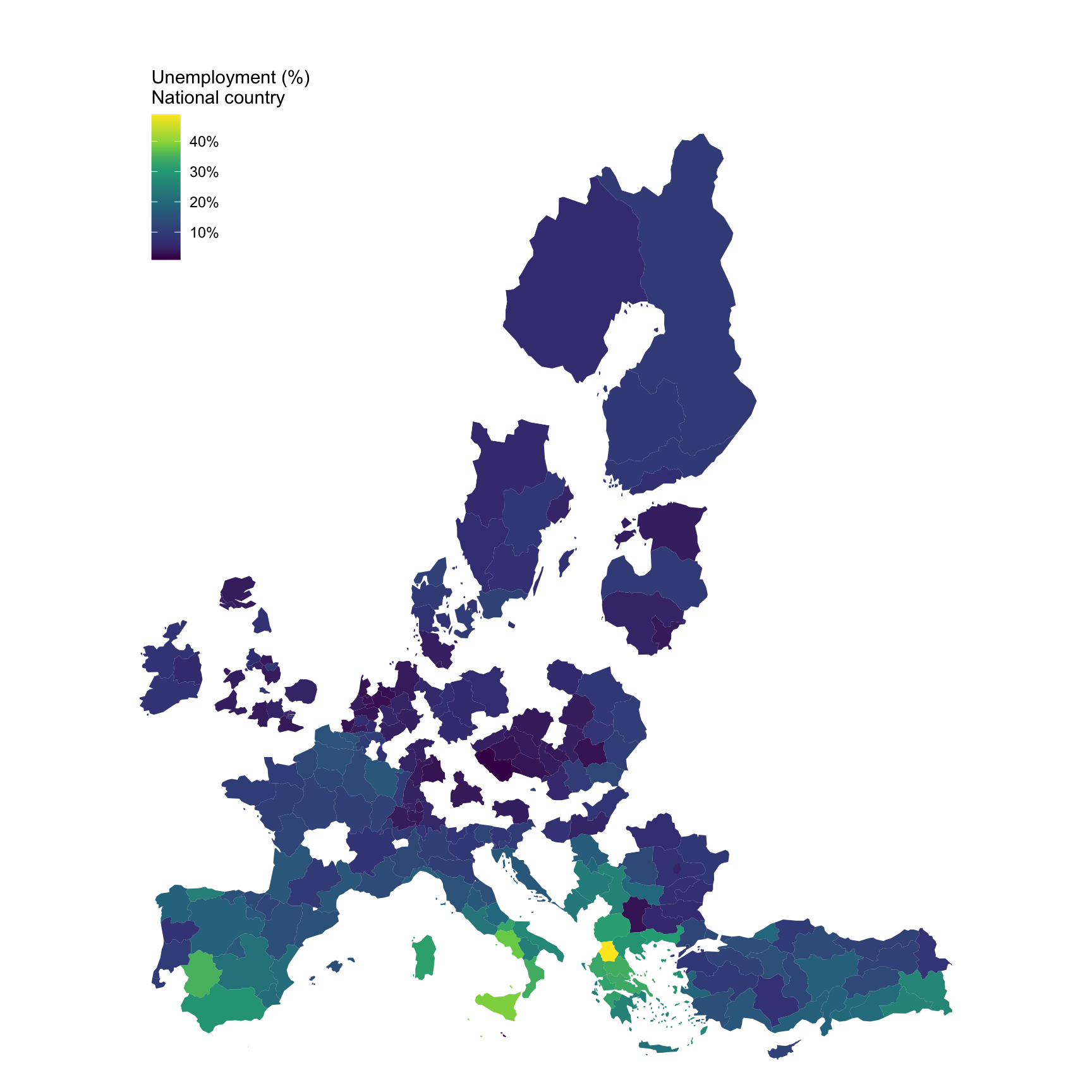
yth_empl_110 %>%
  filter(age == "Y15-29",
         sex == "T",
         nchar(geo) == 4,
         time == "2018") %>%
  right_join(europe_NUTS2, by = "geo") %>%
  filter(long >= -13.5, lat >= 33) %>%
  ggplot(., aes(x = long, y = lat, group = group, fill = values/100)) +
  geom_polygon() + coord_map() +
  scale_fill_viridis_c(na.value = "white",
                       labels = scales::percent_format(accuracy = 1),
                       breaks = 0.01*seq(0, 100, 10),
                       values = c(0, 0.1, 0.3, 0.5, 0.7, 0.8, 1)) +
  theme_void() + theme(legend.position = c(0.15, 0.85)) +
  labs(fill = "Unemployment (%) \nNational country")

Y25-29

Code

yth_empl_110 %>%
  filter(age == "Y25-29",
         sex == "T",
         nchar(geo) == 4,
         time == "2018") %>%
  right_join(europe_NUTS2, by = "geo") %>%
  filter(long >= -13.5, lat >= 33) %>%
  ggplot(., aes(x = long, y = lat, group = group, fill = values/100)) +
  geom_polygon() + coord_map() +
  scale_fill_viridis_c(na.value = "white",
                       labels = scales::percent_format(accuracy = 1),
                       breaks = 0.01*seq(0, 100, 10),
                       values = c(0, 0.1, 0.3, 0.5, 0.7, 0.8, 1)) +
  theme_void() + theme(legend.position = c(0.15, 0.85)) +
  labs(fill = "Unemployment (%) \nNational country")