Last observation: 2025 (N = 30)
First observation: 1995 (N = 30)
Last data update: 06 oct. 2026, 23:30
Last compile: 07 oct. 2026, 01:29
tipslm13 |>
  # CP_MNAC Current prices, million units of national currency
  filter(geo %in% c("FR", "DE", "PT")) |>
  year_to_enddate() |>

  mutate(values = values/100) |>
  add_flag_color("Geo") |>
  ggplot() + geom_line() + theme_minimal()  +
  aes(x = date, y = values, color = color) +
  scale_color_identity() + add_flags +
  scale_x_date(breaks = as.Date(paste0(seq(1960, 2100, 1), "-01-01")),
               labels = date_format("%Y")) +
  theme(legend.position = c(0.3, 0.85),
        legend.title = element_blank()) +
  xlab("") + ylab("Compensation of employees")
tipsna62 |>
  filter(geo %in% c("DE"),
         unit == "THS_PER") |>
  select(geo, time, emp = values) |>
  left_join(tipslm13 |>
              select(geo, time, comp = values),
            by = c("geo", "time")) |>
  left_join(une_rt_a |>
              filter(age == "Y20-64",
                     sex == "T",
                     unit == "PC_ACT") |>
              select(geo, time, unr = values),
            by = c("geo", "time")) |>
  mutate(comp_emp = comp/emp,
         comp_emp_d1 = comp_emp/lag(comp_emp, 1)-1) |>
  year_to_enddate() |>
  transmute(date, comp_emp_d1=100*comp_emp_d1, unr = unr) |>
  gather(variable, value, -date) |>
  mutate(Variable = case_when(variable == "comp_emp_d1" ~ "Wage Inflation (%)",
                              variable == "unr" ~ "Unemployment Rate (%)")) |>
  ggplot() + geom_line() + theme_minimal()  +
  aes(x = date, y = value/100, color = Variable, linetype = Variable) +
  scale_color_manual(values = viridis(3)[1:2]) +
  scale_x_date(breaks = as.Date(paste0(seq(1960, 2100, 1), "-01-01")),
               labels = date_format("%Y")) +
  scale_y_continuous(breaks = 0.01*seq(-100, 100, 1),
                     labels = percent_format(accuracy = 1)) +
  theme(legend.position = c(0.8, 0.85),
        legend.title = element_blank()) +
  xlab("") + ylab("Unemployment Rate, Wage Inflation (%)")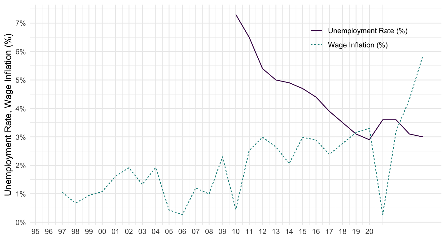
tipsna62 |>
  filter(geo %in% c("FR"),
         unit == "THS_PER") |>
  select(geo, time, emp = values) |>
  left_join(tipslm13 |>
              select(geo, time, comp = values),
            by = c("geo", "time")) |>
  left_join(une_rt_a |>
              filter(age == "Y20-64",
                     sex == "T",
                     unit == "PC_ACT") |>
              select(geo, time, unr = values),
            by = c("geo", "time")) |>
  mutate(comp_emp = comp/emp,
         comp_emp_d1 = comp_emp/lag(comp_emp, 1)-1) |>
  year_to_enddate() |>
  transmute(date, comp_emp_d1=100*comp_emp_d1, unr = unr) |>
  gather(variable, value, -date) |>
  mutate(Variable = case_when(variable == "comp_emp_d1" ~ "Wage Inflation (%)",
                              variable == "unr" ~ "Unemployment Rate (%)")) |>
  ggplot() + geom_line() + theme_minimal()  +
  aes(x = date, y = value/100, color = Variable, linetype = Variable) +
  scale_color_manual(values = viridis(3)[1:2]) +
  scale_x_date(breaks = as.Date(paste0(seq(1960, 2100, 1), "-01-01")),
               labels = date_format("%Y")) +
  scale_y_continuous(breaks = 0.01*seq(-100, 100, 1),
                     labels = percent_format(accuracy = 1)) +
  theme(legend.position = c(0.2, 0.85),
        legend.title = element_blank()) +
  xlab("") + ylab("Unemployment Rate, Wage Inflation (%)")
tipsna62 |>
  filter(geo %in% c("PT"),
         unit == "THS_PER") |>
  select(geo, time, emp = values) |>
  left_join(tipslm13 |>
              select(geo, time, comp = values),
            by = c("geo", "time")) |>
  left_join(une_rt_a |>
              filter(age == "Y20-64",
                     sex == "T",
                     unit == "PC_ACT") |>
              select(geo, time, unr = values),
            by = c("geo", "time")) |>
  mutate(comp_emp = comp/emp,
         comp_emp_d1 = comp_emp/lag(comp_emp, 1)-1) |>
  year_to_enddate() |>
  transmute(date, comp_emp_d1=100*comp_emp_d1, unr = unr) |>
  gather(variable, value, -date) |>
  mutate(Variable = case_when(variable == "comp_emp_d1" ~ "Wage Inflation (%)",
                              variable == "unr" ~ "Unemployment Rate (%)")) |>
  ggplot() + geom_line() + theme_minimal()  +
  aes(x = date, y = value/100, color = Variable, linetype = Variable) +
  scale_color_manual(values = viridis(3)[1:2]) +
  scale_x_date(breaks = as.Date(paste0(seq(1960, 2100, 1), "-01-01")),
               labels = date_format("%Y")) +
  scale_y_continuous(breaks = 0.01*seq(-100, 100, 1),
                     labels = percent_format(accuracy = 1)) +
  theme(legend.position = c(0.2, 0.85),
        legend.title = element_blank()) +
  xlab("") + ylab("Unemployment Rate, Wage Inflation (%)")
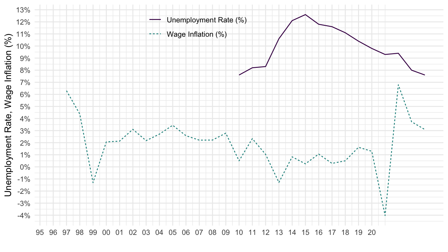
tipsna62 |>
  filter(geo %in% c("ES"),
         unit == "THS_PER") |>
  select(geo, time, emp = values) |>
  left_join(tipslm13 |>
              select(geo, time, comp = values),
            by = c("geo", "time")) |>
  left_join(une_rt_a |>
              filter(age == "Y20-64",
                     sex == "T",
                     unit == "PC_ACT") |>
              select(geo, time, unr = values),
            by = c("geo", "time")) |>
  mutate(comp_emp = comp/emp,
         comp_emp_d1 = comp_emp/lag(comp_emp, 1)-1) |>
  year_to_enddate() |>
  transmute(date, comp_emp_d1=100*comp_emp_d1, unr = unr) |>
  gather(variable, value, -date) |>
  mutate(Variable = case_when(variable == "comp_emp_d1" ~ "Wage Inflation (%)",
                              variable == "unr" ~ "Unemployment Rate (%)")) |>
  ggplot() + geom_line() + theme_minimal()  +
  aes(x = date, y = value/100, color = Variable, linetype = Variable) +
  scale_color_manual(values = viridis(3)[1:2]) +
  scale_x_date(breaks = as.Date(paste0(seq(1960, 2100, 1), "-01-01")),
               labels = date_format("%Y")) +
  scale_y_continuous(breaks = 0.01*seq(-100, 100, 1),
                     labels = percent_format(accuracy = 1)) +
  theme(legend.position = c(0.2, 0.85),
        legend.title = element_blank()) +
  xlab("") + ylab("Unemployment Rate, Wage Inflation (%)")
tipsna62 |>
  filter(geo %in% c("IT"),
         unit == "THS_PER") |>
  select(geo, time, emp = values) |>
  left_join(tipslm13 |>
              select(geo, time, comp = values),
            by = c("geo", "time")) |>
  left_join(une_rt_a |>
              filter(age == "Y20-64",
                     sex == "T",
                     unit == "PC_ACT") |>
              select(geo, time, unr = values),
            by = c("geo", "time")) |>
  mutate(comp_emp = comp/emp,
         comp_emp_d1 = comp_emp/lag(comp_emp, 1)-1) |>
  year_to_enddate() |>
  transmute(date, comp_emp_d1=100*comp_emp_d1, unr = unr) |>
  gather(variable, value, -date) |>
  mutate(Variable = case_when(variable == "comp_emp_d1" ~ "Wage Inflation (%)",
                              variable == "unr" ~ "Unemployment Rate (%)")) |>
  ggplot() + geom_line() + theme_minimal()  +
  aes(x = date, y = value/100, color = Variable, linetype = Variable) +
  scale_color_manual(values = viridis(3)[1:2]) +
  scale_x_date(breaks = as.Date(paste0(seq(1960, 2100, 1), "-01-01")),
               labels = date_format("%Y")) +
  scale_y_continuous(breaks = 0.01*seq(-100, 100, 1),
                     labels = percent_format(accuracy = 1)) +
  theme(legend.position = c(0.4, 0.9),
        legend.title = element_blank()) +
  xlab("") + ylab("Unemployment Rate, Wage Inflation (%)")