Code
tibble(LAST_DOWNLOAD = as.Date(file.info("~/iCloud/website/data/eurostat/sts_inlb_m.RData")$mtime)) %>%
print_table_conditional()| LAST_DOWNLOAD |
|---|
| 2026-04-14 |
Data - Eurostat
tibble(LAST_DOWNLOAD = as.Date(file.info("~/iCloud/website/data/eurostat/sts_inlb_m.RData")$mtime)) %>%
print_table_conditional()| LAST_DOWNLOAD |
|---|
| 2026-04-14 |
| LAST_COMPILE |
|---|
| 2026-07-22 |
sts_inlb_m %>%
  group_by(time) %>%
  summarise(Nobs = n()) %>%
  arrange(desc(time)) %>%
  head(1) %>%
print_table_conditional()| time | Nobs |
|---|---|
| 2026M02 | 1478 |
sts_inlb_m %>%
  left_join(nace_r2, by = "nace_r2") %>%
  group_by(nace_r2, Nace_r2) %>%
  summarise(Nobs = n()) %>%
{if (is_html_output()) datatable(., filter = 'top', rownames = F) else .}sts_inlb_m %>%
left_join(s_adj, by = "s_adj") %>%
group_by(s_adj, S_adj) %>%
summarise(Nobs = n()) %>%
arrange(-Nobs) %>%
{if (is_html_output()) print_table(.) else .}| s_adj | S_adj | Nobs |
|---|---|---|
| SCA | Seasonally and calendar adjusted data | 935795 |
| NSA | Unadjusted data (i.e. neither seasonally adjusted nor calendar adjusted data) | 814845 |
| CA | Calendar adjusted data, not seasonally adjusted data | 586185 |
sts_inlb_m %>%
  left_join(unit, by = "unit") %>%
  group_by(unit, Unit) %>%
  summarise(Nobs = n()) %>%
  arrange(-Nobs) %>%
{if (is_html_output()) print_table(.) else .}| unit | Unit | Nobs |
|---|---|---|
| I15 | Index, 2015=100 | 671160 |
| I21 | Index, 2021=100 | 667477 |
| I10 | Index, 2010=100 | 398731 |
| PCH_SM | Percentage change compared to same period in previous year | 330926 |
| PCH_PRE | Percentage change on previous period | 268531 |
sts_inlb_m %>%
  left_join(indic_bt, by = "indic_bt") %>%
  group_by(indic_bt, Indic_bt) %>%
  summarise(Nobs = n()) %>%
  arrange(-Nobs) %>%
{if (is_html_output()) print_table(.) else .}| indic_bt | Indic_bt | Nobs |
|---|---|---|
| WAGE | Wages and salaries | 1018662 |
| HW | Hours worked by employees | 777865 |
| EMP | Persons employed | 540298 |
sts_inlb_m %>%
  left_join(geo, by = "geo") %>%
  group_by(geo, Geo) %>%
  summarise(Nobs = n()) %>%
  arrange(-Nobs) %>%
  mutate(Geo = ifelse(geo == "DE", "Germany", Geo)) %>%
  mutate(Flag = gsub(" ", "-", str_to_lower(Geo)),
         Flag = paste0('<img src="../../bib/flags/vsmall/', Flag, '.png" alt="Flag">')) %>%
  select(Flag, everything()) %>%
{if (is_html_output()) datatable(., filter = 'top', rownames = F, escape = F) else .}sts_inlb_m %>%
group_by(time) %>%
summarise(Nobs = n()) %>%
{if (is_html_output()) datatable(., filter = 'top', rownames = F) else .}sts_inlb_m %>%
filter(nace_r2 == "C",
geo %in% c("FR", "DE", "IT"),
s_adj == "SCA",
unit == "I15") %>%
select(geo, indic_bt, time, values) %>%
group_by(indic_bt) %>%
mutate(values = 100*values/values[time == "2000M01"]) %>%
left_join(indic_bt, by = "indic_bt") %>%
month_to_date %>%
ggplot() + ylab("") + xlab("") + theme_minimal() +
geom_line(aes(x = date, y = values, color = Indic_bt)) +
scale_color_manual(values = viridis(4)[1:3]) +
scale_x_date(breaks = seq(1920, 2025, 2) %>% paste0("-01-01") %>% as.Date,
labels = date_format("%y")) +
theme(legend.position = c(0.25, 0.85),
legend.title = element_blank()) +
scale_y_log10(breaks = seq(-60, 300, 10))
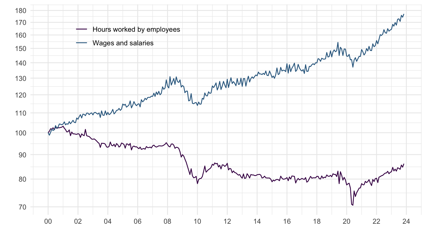
sts_inlb_m %>%
  filter(nace_r2 == "C",
         geo %in% c("PT"),
         s_adj == "SCA",
         unit == "I15") %>%
  select(geo, indic_bt, time, values) %>%
  group_by(indic_bt) %>%
  mutate(values = 100*values/values[time == "2000M01"]) %>%
  left_join(indic_bt, by = "indic_bt") %>%
  month_to_date %>%
  ggplot() + ylab("") + xlab("") + theme_minimal() +
  geom_line(aes(x = date, y = values, color = Indic_bt)) +
  scale_color_manual(values = viridis(4)[1:3]) +
  scale_x_date(breaks = seq(1920, 2025, 2) %>% paste0("-01-01") %>% as.Date,
               labels = date_format("%y")) +
  theme(legend.position = c(0.25, 0.85),
        legend.title = element_blank()) +
  scale_y_log10(breaks = seq(-60, 300, 10))
sts_inlb_m %>%
  filter(nace_r2 == "C",
         geo %in% c("AT"),
         s_adj == "SCA",
         unit == "I15") %>%
  select(geo, indic_bt, time, values) %>%
  group_by(indic_bt) %>%
  mutate(values = 100*values/values[time == "2000M01"]) %>%
  left_join(indic_bt, by = "indic_bt") %>%
  month_to_date %>%
  ggplot() + ylab("") + xlab("") + theme_minimal() +
  geom_line(aes(x = date, y = values, color = Indic_bt)) +
  scale_color_manual(values = viridis(4)[1:3]) +
  scale_x_date(breaks = seq(1920, 2025, 2) %>% paste0("-01-01") %>% as.Date,
               labels = date_format("%y")) +
  theme(legend.position = c(0.25, 0.85),
        legend.title = element_blank()) +
  scale_y_log10(breaks = seq(-60, 300, 10))
sts_inlb_m %>%
  filter(nace_r2 == "C",
         geo %in% c("SE"),
         s_adj == "SCA",
         unit == "I15") %>%
  select(geo, indic_bt, time, values) %>%
  group_by(indic_bt) %>%
  mutate(values = 100*values/values[time == "2000M01"]) %>%
  left_join(indic_bt, by = "indic_bt") %>%
  month_to_date %>%
  ggplot() + ylab("") + xlab("") + theme_minimal() +
  geom_line(aes(x = date, y = values, color = Indic_bt)) +
  scale_color_manual(values = viridis(4)[1:3]) +
  scale_x_date(breaks = seq(1920, 2025, 2) %>% paste0("-01-01") %>% as.Date,
               labels = date_format("%y")) +
  theme(legend.position = c(0.25, 0.85),
        legend.title = element_blank()) +
  scale_y_log10(breaks = seq(-60, 300, 10))