Last observation: août 2026 (N = 562)
First observation: janv. 1980 (N = 4)
Last data update: 24 oct. 2026, 00:34
Last compile: 24 oct. 2026, 01:42
sts_copr_m |>
  filter(nace_r2 == "F",
         unit == "I21",
         geo %in% c("FR", "DE", "IT"),
         s_adj == "SCA") |>
  select(geo, Geo, time, values) |>
  group_by(geo) |>
  mutate(values = 100*values/values[time == "1997M01"]) |>

  mutate(Geo = ifelse(geo == "DE", "Germany", Geo)) |>
  month_to_date() |>
  add_flag_color("Geo") |>
  ggplot() + ylab("Construction Production") + xlab("") + theme_minimal() +
  geom_line(aes(x = date, y = values, color = color)) +
  scale_color_identity() + add_flags +
  scale_color_manual(values = c("#0055a4", "#000000", "#008c45")) +
  scale_x_date(breaks = seq(1920, 2100, 2) |> paste0("-01-01") |> as.Date(),
               labels = date_format("%Y")) +
  geom_image(data = . %>%
               filter(date == as.Date("2007-01-01")) %>%
               mutate(date = as.Date("2007-01-01"),
                      image = paste0("../../icon/flag/", str_to_lower(Geo), ".png")),
             aes(x = date, y = values, image = image), asp = 1.5) +
  theme(legend.position = "none") +
  scale_y_log10(breaks = seq(-60, 300, 10))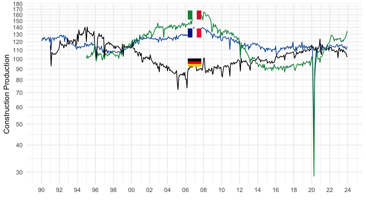
sts_copr_m |>
  filter(nace_r2 == "F",
         unit == "I21",
         s_adj == "SCA",
         time %in% c("2019M11", "2020M02", "2020M03", "2020M04", "2020M05", "2020M08", "2020M11"),
         !(geo %in% c("IE", "EU28"))) |>
  select(geo, Geo, time, values) |>
  group_by(geo) |>
  mutate(values = 100*values/values[time == "2019M11"]) |>

  spread(time, values) |>
  mutate(Geo = ifelse(geo == "DE", "Germany", Geo)) |>
  mutate(Flag = gsub(" ", "-", str_to_lower(Geo)),
         Flag = paste0('<img src="../../bib/flags/vsmall/', Flag, '.png" alt="Flag">')) |>
  select(Flag, everything()) |>
  arrange(`2020M04`) %>%
{if (is_html_output()) datatable(., filter = 'top', rownames = F, escape = F) else .}sts_copr_m |>
filter(nace_r2 == "F",
unit == "I21",
geo %in% c("FR", "DE", "IT"),
s_adj == "SCA") |>
select(geo, Geo, time, values) |>
group_by(geo) |>
mutate(values = 100*values/values[time == "2018M01"]) |>
mutate(Geo = ifelse(geo == "DE", "Germany", Geo)) |>
month_to_date() |>
filter(date >= as.Date("2018-01-01")) |>
add_flag_color("Geo") |>
ggplot() + ylab("Construction Production") + xlab("") + theme_minimal() +
geom_line(aes(x = date, y = values, color = color)) +
scale_color_identity() + add_flags +
scale_color_manual(values = c("#0055a4", "#000000", "#008c45")) +
scale_x_date(breaks = "3 months",
labels = date_format("%b %Y")) +
geom_image(data = . %>%
filter(date == as.Date("2020-08-01")) %>%
mutate(image = paste0("../../icon/flag/", str_to_lower(Geo), ".png")),
aes(x = date, y = values, image = image), asp = 1.5) +
theme(legend.position = "none") +
scale_y_log10(breaks = seq(-60, 300, 10))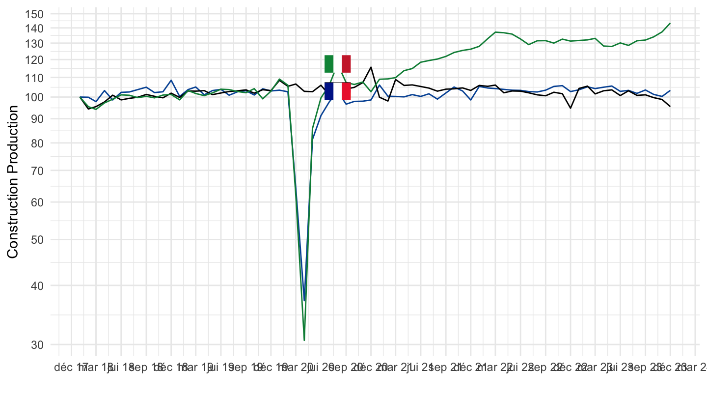
sts_copr_m |>
  filter(nace_r2 == "F",
         unit == "I21",
         geo %in% c("FR", "DE", "IT"),
         s_adj == "SCA") |>
  select(geo, Geo, time, values) |>
  group_by(geo) |>
  mutate(values = 100*values/values[time == "2019M09"]) |>

  mutate(Geo = ifelse(geo == "DE", "Germany", Geo)) |>
  month_to_date() |>
  filter(date >= as.Date("2019-09-01")) |>
  add_flag_color("Geo") |>
  ggplot() + ylab("Construction Production") + xlab("") + theme_minimal() +
  geom_line(aes(x = date, y = values, color = color)) +
  scale_color_identity() + add_flags +
  scale_color_manual(values = c("#0055a4", "#000000", "#008c45")) +
  scale_x_date(breaks = "2 months",
               labels = date_format("%b %Y")) +
  geom_image(data = . %>%
               filter(date == as.Date("2020-08-01")) %>%
               mutate(image = paste0("../../icon/flag/", str_to_lower(Geo), ".png")),
             aes(x = date, y = values, image = image), asp = 1.5) +
  theme(legend.position = "none") +
  scale_y_log10(breaks = seq(-60, 300, 10))
sts_copr_m |>
  filter(nace_r2 == "F",
         unit == "I21",
         geo %in% c("FR", "DE", "IT", "ES"),
         s_adj == "SCA") |>
  select(geo, Geo, time, values) |>
  group_by(geo) |>
  mutate(values = 100*values/values[time == "2020M02"]) |>

  mutate(Geo = ifelse(geo == "DE", "Germany", Geo)) |>
  month_to_date() |>
  filter(date >= as.Date("2020-02-01")) |>
  add_flag_color("Geo") |>
  ggplot() + ylab("Construction Production") + xlab("") + theme_minimal() +
  geom_line(aes(x = date, y = values, color = color)) +
  scale_color_identity() + add_flags +
  scale_color_manual(values = c("#0055a4", "#000000", "#008c45", "#C60B1E")) +
  scale_x_date(breaks = "1 month",
               labels = date_format("%b %Y")) +
  geom_image(data = . %>%
               filter(date == as.Date("2020-08-01")) %>%
               mutate(image = paste0("../../icon/flag/", str_to_lower(Geo), ".png")),
             aes(x = date, y = values, image = image), asp = 1.5) +
  theme(legend.position = "none") +
  scale_y_log10(breaks = seq(-60, 300, 10))
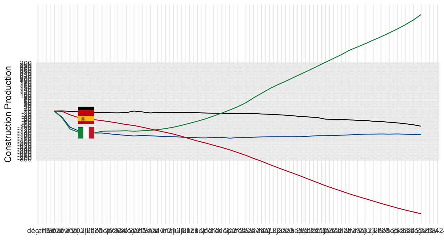
sts_copr_m |>
  filter(nace_r2 == "F",
         unit == "I21",
         geo %in% c("FR", "DE", "IT", "ES"),
         s_adj == "SCA") |>
  select(geo, Geo, time, values) |>
  group_by(geo) |>
  mutate(values = 100*values/values[time == "2020M02"]) |>

  month_to_date() |>
  filter(date >= as.Date("2020-02-01")) |>
  group_by(Geo) |>
  arrange(date) |>
  mutate(values = values-100,
         values = cumsum(values)) |>
  add_flag_color("Geo") |>
  ggplot() + ylab("Construction Production") + xlab("") + theme_minimal() +
  geom_line(aes(x = date, y = values, color = color)) +
  scale_color_identity() + add_flags +
  scale_color_manual(values = c("#0055a4", "#000000", "#008c45", "#C60B1E")) +
  scale_x_date(breaks = "1 month",
               labels = date_format("%b %Y")) +
  geom_image(data = . %>%
               filter(date == as.Date("2020-06-01")) %>%
               mutate(image = paste0("../../icon/flag/", str_to_lower(Geo), ".png")),
             aes(x = date, y = values, image = image), asp = 1.5) +
  theme(legend.position = "none") +
  scale_y_continuous(breaks = seq(-300, 300, 10))