| LAST_COMPILE |
|---|
| 2026-03-24 |
Pensions - spr_exp_pens
Data - Eurostat
Info
LAST_COMPILE
Last
Code
spr_exp_pens %>%
  group_by(time) %>%
  summarise(Nobs = n()) %>%
  arrange(desc(time)) %>%
  head(1) %>%
print_table_conditional()| time | Nobs |
|---|---|
| 2023 | 7942 |
spdepb
Code
spr_exp_pens %>%
  left_join(spdepb, by = "spdepb") %>%
  group_by(spdepb, Spdepb) %>%
  summarise(Nobs = n()) %>%
  arrange(-Nobs) %>%
print_table_conditional| spdepb | Spdepb | Nobs |
|---|---|---|
| TOTAL | Total | 33038 |
| OLD | NA | 32983 |
| SRV | NA | 32774 |
| DIS | NA | 32752 |
| AOLD | NA | 30949 |
| ERLM | NA | 30179 |
| ERRC | NA | 29191 |
| PART | NA | 29134 |
spdepm
Code
spr_exp_pens %>%
  left_join(spdepm, by = "spdepm") %>%
  group_by(spdepm, Spdepm) %>%
  summarise(Nobs = n()) %>%
  arrange(-Nobs) %>%
print_table_conditional| spdepm | Spdepm | Nobs |
|---|---|---|
| TOTAL | Total | 84977 |
| NMT | NA | 84878 |
| MT | NA | 81145 |
unit
Code
spr_exp_pens %>%
  left_join(unit, by = "unit") %>%
  group_by(unit, Unit) %>%
  summarise(Nobs = n()) %>%
  arrange(-Nobs) %>%
print_table_conditional| unit | Unit | Nobs |
|---|---|---|
| MIO_EUR | Million euro | 27505 |
| MIO_PPS | Million purchasing power standards (PPS) | 24118 |
| PC_GDP | Percentage of gross domestic product (GDP) | 23110 |
| MEUR_KP10 | Million euro (at constant 2010 prices) | 22870 |
| MEUR_KP15 | NA | 22870 |
| MIO_NAC | Million units of national currency | 22369 |
| PPS_HAB | Purchasing power standard (PPS) per inhabitant | 22230 |
| EUR_HAB_KP10 | Euro per inhabitant (at constant 2010 prices) | 22134 |
| EUR_HAB_KP15 | NA | 22134 |
| MNAC_KP10 | Million units of national currency at constant 2010 prices | 20830 |
| MNAC_KP15 | NA | 20830 |
geo
Code
spr_exp_pens %>%
  left_join(geo, by = "geo") %>%
  group_by(geo, Geo) %>%
  summarise(Nobs = n()) %>%
  arrange(-Nobs) %>%
  mutate(Flag = gsub(" ", "-", str_to_lower(Geo)),
         Flag = paste0('<img src="../../icon/flag/vsmall/', Flag, '.png" alt="Flag">')) %>%
  select(Flag, everything()) %>%
  {if (is_html_output()) datatable(., filter = 'top', rownames = F, escape = F) else .}
List of Countries: 2000-2019
Code
spr_exp_pens %>%
  filter(# OLD: Old age pension
         spdepb == "TOTAL",
         # TOTAL: Total
         spdepm == "TOTAL",
         # MIO_EUR: Million euro
         unit == "PC_GDP",
         time %in% c("1997", "2017")) %>%
  select(geo, time, values) %>%
  left_join(geo, by = "geo") %>%
  spread(time, values) %>%
  mutate(`Change` = round(`2017` - `1997`, 1)) %>%
  na.omit %>%
  arrange(Change) %>%
  mutate(Flag = gsub(" ", "-", str_to_lower(Geo)),
         Flag = paste0('<img src="../../icon/flag/vsmall/', Flag, '.png" alt="Flag">')) %>%
  select(Flag, everything()) %>%
  {if (is_html_output()) datatable(., filter = 'top', rownames = F, escape = F) else .}
France, Germany, Italy
% of GDP - Total
Code
spr_exp_pens %>%
  filter(geo %in% c("FR", "DE", "IT"),
         # OLD: Old age pension
         spdepb == "TOTAL",
         # TOTAL: Total
         spdepm == "TOTAL",
         # MIO_EUR: Million euro
         unit == "PC_GDP") %>%
  year_to_date %>%
  left_join(geo, by = "geo") %>%
  mutate(values = values/100) %>%
  ggplot + geom_line(aes(x = date, y = values, color = Geo)) +
  scale_color_manual(values = c("#002395", "#000000", "#009246")) +
  theme_minimal()  + add_flags +
  scale_x_date(breaks = as.Date(paste0(seq(1960, 2100, 2), "-01-01")),
               labels = date_format("%Y")) +
  theme(legend.position = "none") +
  xlab("") + ylab("Total Spending on Pensions (% of GDP)") +
  scale_y_continuous(breaks = 0.01*seq(0, 60, 1),
                     labels = scales::percent_format(accuracy = 1))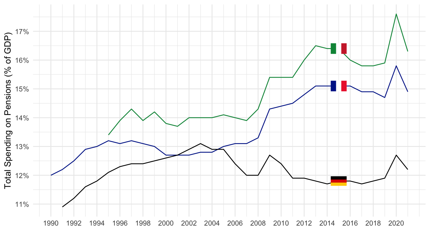
% of GDP - Old age pension
Code
spr_exp_pens %>%
  filter(geo %in% c("FR", "DE", "IT"),
         # OLD: Old age pension
         spdepb == "OLD",
         # TOTAL: Total
         spdepm == "TOTAL",
         # PC_GDP: Million euro
         unit == "PC_GDP") %>%
  year_to_date %>%
  left_join(geo, by = "geo") %>%
  mutate(values = values/100) %>%
  ggplot + geom_line(aes(x = date, y = values, color = Geo)) +
  scale_color_manual(values = c("#002395", "#000000", "#009246")) +
  theme_minimal()  + add_flags +
  scale_x_date(breaks = as.Date(paste0(seq(1960, 2100, 2), "-01-01")),
               labels = date_format("%Y")) +
  theme(legend.position = c(0.3, 0.85),
        legend.title = element_blank()) +
  xlab("") + ylab("Old Age Pension (% of GDP)") +
  scale_y_continuous(breaks = 0.01*seq(0, 60, 1),
                     labels = scales::percent_format(accuracy = 1))
Amounts (Bn€) - Total
Code
spr_exp_pens %>%
  filter(geo %in% c("FR", "DE", "IT"),
         # OLD: Old age pension
         spdepb == "TOTAL",
         # TOTAL: Total
         spdepm == "TOTAL",
         # MIO_EUR: Million euro
         unit == "MIO_EUR") %>%
  year_to_date %>%
  left_join(geo, by = "geo") %>%
  mutate(values = values/1000) %>%
  ggplot + geom_line(aes(x = date, y = values, color = Geo)) +
  scale_color_manual(values = c("#002395", "#000000", "#009246")) +
  theme_minimal()  + add_flags +
  scale_x_date(breaks = as.Date(paste0(seq(1960, 2100, 2), "-01-01")),
               labels = date_format("%Y")) +
  theme(legend.position = "none") +
  xlab("") + ylab("") +
  scale_y_log10(breaks = seq(0, 1000, 50),
                labels = dollar_format(suffix = " Bn€", prefix = "", accuracy = 1))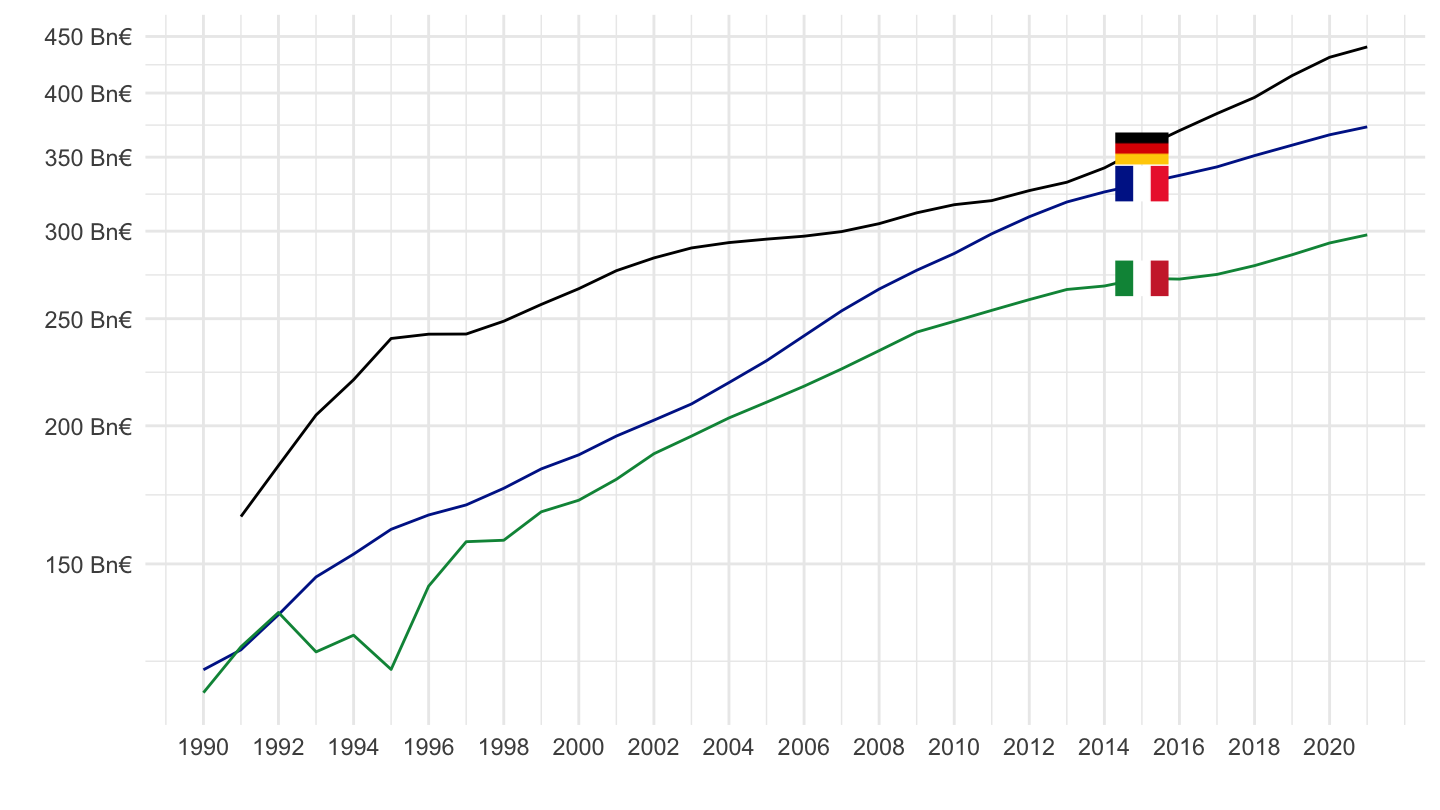
Amounts (Bn€) - Old age pension
Code
spr_exp_pens %>%
  filter(geo %in% c("FR", "DE", "IT"),
         # OLD: Old age pension
         spdepb == "OLD",
         # TOTAL: Total
         spdepm == "TOTAL",
         # MIO_EUR: Million euro
         unit == "MIO_EUR") %>%
  year_to_date %>%
  left_join(geo, by = "geo") %>%
  mutate(values = values/1000) %>%
  ggplot + geom_line(aes(x = date, y = values, color = Geo)) +
  scale_color_manual(values = c("#002395", "#000000", "#009246")) +
  theme_minimal()  + add_flags +
  scale_x_date(breaks = as.Date(paste0(seq(1960, 2100, 2), "-01-01")),
               labels = date_format("%Y")) +
  theme(legend.position = "none") +
  xlab("") + ylab("") +
  scale_y_log10(breaks = seq(0, 1000, 50),
                labels = dollar_format(suffix = " Bn€", prefix = "", accuracy = 1))
Austria, Denmark, Netherlands, Sweden
% of GDP - Total
Code
spr_exp_pens %>%
  filter(geo %in% c("AT", "DK", "NL", "SE"),
         # OLD: Old age pension
         spdepb == "TOTAL",
         # TOTAL: Total
         spdepm == "TOTAL",
         # MIO_EUR: Million euro
         unit == "PC_GDP") %>%
  year_to_date %>%
  left_join(geo, by = "geo") %>%
  left_join(colors, by = c("Geo" = "country")) %>%
  mutate(values = values/100) %>%
  ggplot + geom_line(aes(x = date, y = values, color = color)) +
  scale_color_identity() + theme_minimal()  + add_flags +
  scale_x_date(breaks = as.Date(paste0(seq(1960, 2100, 2), "-01-01")),
               labels = date_format("%Y")) +
  theme(legend.position = c(0.1, 0.85),
        legend.title = element_blank()) +
  xlab("") + ylab("Total Spending on Pensions (% of GDP)") +
  scale_y_continuous(breaks = 0.01*seq(0, 60, 1),
                     labels = scales::percent_format(accuracy = 1))
France, Germany, Italy, Sweden
Total
Code
spr_exp_pens %>%
  filter(geo %in% c("FR", "DE", "IT", "SE"),
         # OLD: Old age pension
         spdepb == "TOTAL",
         # TOTAL: Total
         spdepm == "TOTAL",
         # MIO_EUR: Million euro
         unit == "PC_GDP") %>%
  year_to_date %>%
  left_join(geo, by = "geo") %>%
  mutate(values = values/100) %>%
  ggplot + geom_line(aes(x = date, y = values, color = Geo)) +
  scale_color_manual(values = c("#002395", "#000000", "#009246", "#FECC00")) +
  theme_minimal()  + add_flags +
  scale_x_date(breaks = as.Date(paste0(seq(1960, 2100, 2), "-01-01")),
               labels = date_format("%Y")) +
  theme(legend.position = "none") +
  xlab("") + ylab("Total Spending on Pensions (% of GDP)") +
  scale_y_continuous(breaks = 0.01*seq(0, 60, 1),
                     labels = scales::percent_format(accuracy = 1))
France, Germany, Italy, Sweden, Greece
Total
Code
spr_exp_pens %>%
  filter(geo %in% c("FR", "DE", "IT", "SE", "EL"),
         # OLD: Old age pension
         spdepb == "TOTAL",
         # TOTAL: Total
         spdepm == "TOTAL",
         # MIO_EUR: Million euro
         unit == "PC_GDP") %>%
  year_to_date %>%
  left_join(geo, by = "geo") %>%
  mutate(values = values/100) %>%
  ggplot + geom_line(aes(x = date, y = values, color = Geo)) +
  scale_color_manual(values = c("#002395", "#000000", "#0D5EAF", "#009246", "#FECC00")) +
  theme_minimal()  + add_flags +
  scale_x_date(breaks = as.Date(paste0(seq(1960, 2100, 2), "-01-01")),
               labels = date_format("%Y")) +
  theme(legend.position = "none") +
  xlab("") + ylab("Total Spending on Pensions (% of GDP)") +
  scale_y_continuous(breaks = 0.01*seq(0, 60, 1),
                     limits = c(0.09, 0.18),
                     labels = scales::percent_format(accuracy = 1))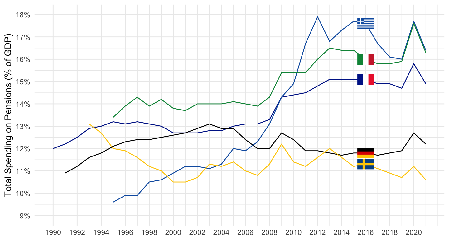
France, Germany, Italy, Greece, Portugal
Total
Code
spr_exp_pens %>%
  filter(geo %in% c("FR", "DE", "IT", "EL", "PT"),
         # OLD: Old age pension
         spdepb == "TOTAL",
         # TOTAL: Total
         spdepm == "TOTAL",
         # MIO_EUR: Million euro
         unit == "PC_GDP") %>%
  year_to_date %>%
  left_join(geo, by = "geo") %>%
  mutate(values = values/100) %>%
  ggplot + geom_line(aes(x = date, y = values, color = Geo)) +
  scale_color_manual(values = c("#002395", "#000000", "#0D5EAF", "#009246", "#FF0000")) +
  theme_minimal()  + add_flags +
  scale_x_date(breaks = as.Date(paste0(seq(1960, 2100, 2), "-01-01")),
               labels = date_format("%Y")) +
  theme(legend.position = "none") +
  xlab("") + ylab("Total Spending on Pensions (% of GDP)") +
  scale_y_continuous(breaks = 0.01*seq(0, 60, 1),
                     labels = scales::percent_format(accuracy = 1))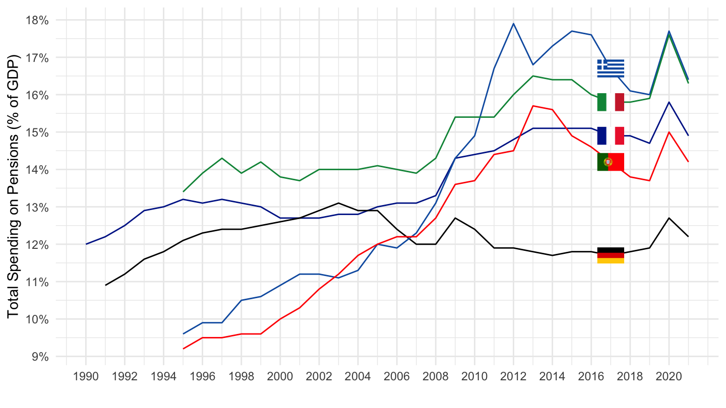
Old age pension
Code
spr_exp_pens %>%
  filter(geo %in% c("FR", "DE", "IT", "EL", "PT"),
         # OLD: Old age pension
         spdepb == "OLD",
         # TOTAL: Total
         spdepm == "TOTAL",
         # MIO_EUR: Million euro
         unit == "PC_GDP") %>%
  year_to_date %>%
  left_join(geo, by = "geo") %>%
  mutate(values = values/100) %>%
  ggplot + geom_line(aes(x = date, y = values, color = Geo)) +
  scale_color_manual(values = c("#002395", "#000000", "#0D5EAF", "#009246", "#FF0000")) +
  theme_minimal()  + add_flags +
  scale_x_date(breaks = as.Date(paste0(seq(1960, 2100, 2), "-01-01")),
               labels = date_format("%Y")) +
  theme(legend.position = "none") +
  xlab("") + ylab("Old age pension (% of GDP)") +
  scale_y_continuous(breaks = 0.01*seq(0, 60, 1),
                     labels = scales::percent_format(accuracy = 1))
Disability pension
Code
spr_exp_pens %>%
  filter(geo %in% c("FR", "DE", "IT", "EL", "PT"),
         # OLD: Old age pension
         spdepb == "DIS",
         # TOTAL: Total
         spdepm == "TOTAL",
         # MIO_EUR: Million euro
         unit == "PC_GDP") %>%
  year_to_date %>%
  left_join(geo, by = "geo") %>%
  mutate(values = values/100) %>%
  ggplot + geom_line(aes(x = date, y = values, color = Geo)) +
  scale_color_manual(values = c("#002395", "#000000", "#0D5EAF", "#009246", "#FF0000")) +
  theme_minimal()  + add_flags +
  scale_x_date(breaks = as.Date(paste0(seq(1960, 2100, 2), "-01-01")),
               labels = date_format("%Y")) +
  theme(legend.position = "none") +
  xlab("") + ylab("Disability pension (% of GDP)") +
  scale_y_continuous(breaks = 0.01*seq(0, 60, 0.2),
                     labels = scales::percent_format(accuracy = .1))
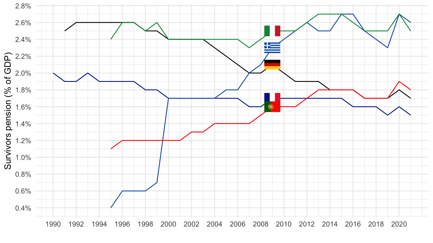
Survivors pension
Code
spr_exp_pens %>%
  filter(geo %in% c("FR", "DE", "IT", "EL", "PT"),
         # OLD: Old age pension
         spdepb == "SRV",
         # TOTAL: Total
         spdepm == "TOTAL",
         # MIO_EUR: Million euro
         unit == "PC_GDP") %>%
  year_to_date %>%
  left_join(geo, by = "geo") %>%
  mutate(values = values/100) %>%
  ggplot + geom_line(aes(x = date, y = values, color = Geo)) +
  scale_color_manual(values = c("#002395", "#000000", "#0D5EAF", "#009246", "#FF0000")) +
  theme_minimal()  + add_flags +
  scale_x_date(breaks = as.Date(paste0(seq(1960, 2100, 2), "-01-01")),
               labels = date_format("%Y")) +
  theme(legend.position = "none") +
  xlab("") + ylab("Survivors pension (% of GDP)") +
  scale_y_continuous(breaks = 0.01*seq(0, 60, 0.2),
                     labels = scales::percent_format(accuracy = .1))