Environmental protection expenditure by size class (NACE Rev. 2, B-E) - sbs_env_sc_r2

Data - Eurostat

Author

François Geerolf

Info

Last observation: 2018 (N = 5382)

First observation: 2008 (N = 5043)

Last data update: 15 juil. 2026, 00:04. Last compile: 02 sept. 2026, 00:54

Structure

Pollution Control Investment, Manufacturing

France, Germany, Italy, Spain

Code

sbs_env_sc_r2 |>
  filter(geo %in% c("FR", "DE", "IT", "ES"),
         nace_r2 == "C",
         size_emp == "TOTAL",
         indic_sb == "V21110") |>
  year_to_date() |>

  left_join(colors, by = c("Geo" = "country")) |>
  ggplot() + geom_line(aes(x = date, y = values, color = color)) +
  theme_minimal() + scale_color_identity() + add_flags +
  scale_x_date(breaks = as.Date(paste0(seq(2005, 2100, 1), "-01-01")),
               labels = date_format("%Y")) +
  xlab("") + ylab("Investment in pollution control equipment (Mn€)")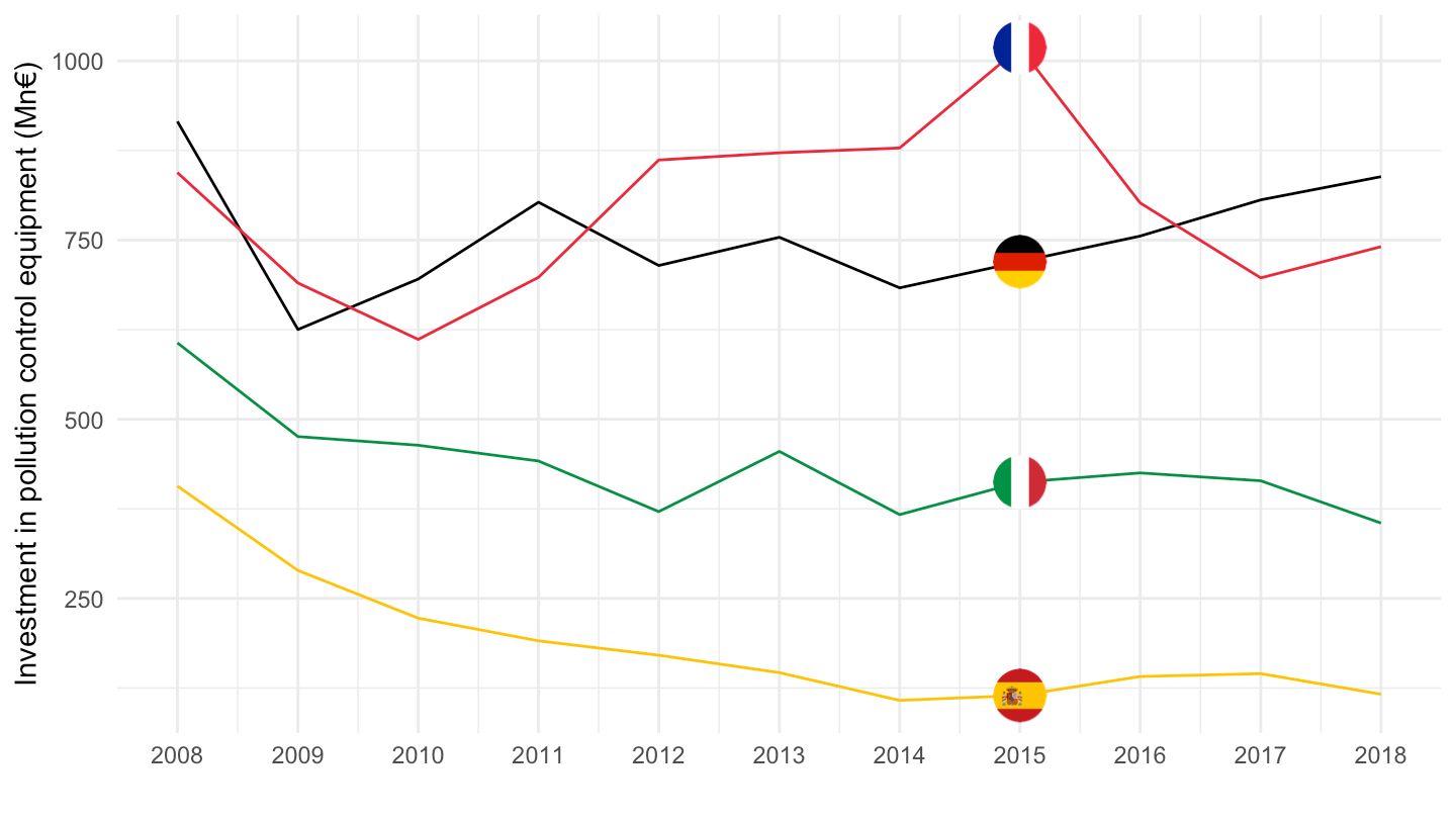

France: Pollution Control vs. Cleaner Technology

Manufacturing

Code

sbs_env_sc_r2 |>
  filter(geo == "FR",
         nace_r2 == "C",
         size_emp == "TOTAL") |>
  year_to_date() |>
  ggplot() + geom_line(aes(x = date, y = values, color = Indic_sb)) +
  theme_minimal() +
  scale_x_date(breaks = as.Date(paste0(seq(2005, 2100, 1), "-01-01")),
               labels = date_format("%Y")) +
  xlab("") + ylab("Investment (Mn€)") +
  theme(legend.position = "bottom", legend.title = element_blank()) +
  guides(color = guide_legend(nrow = 2))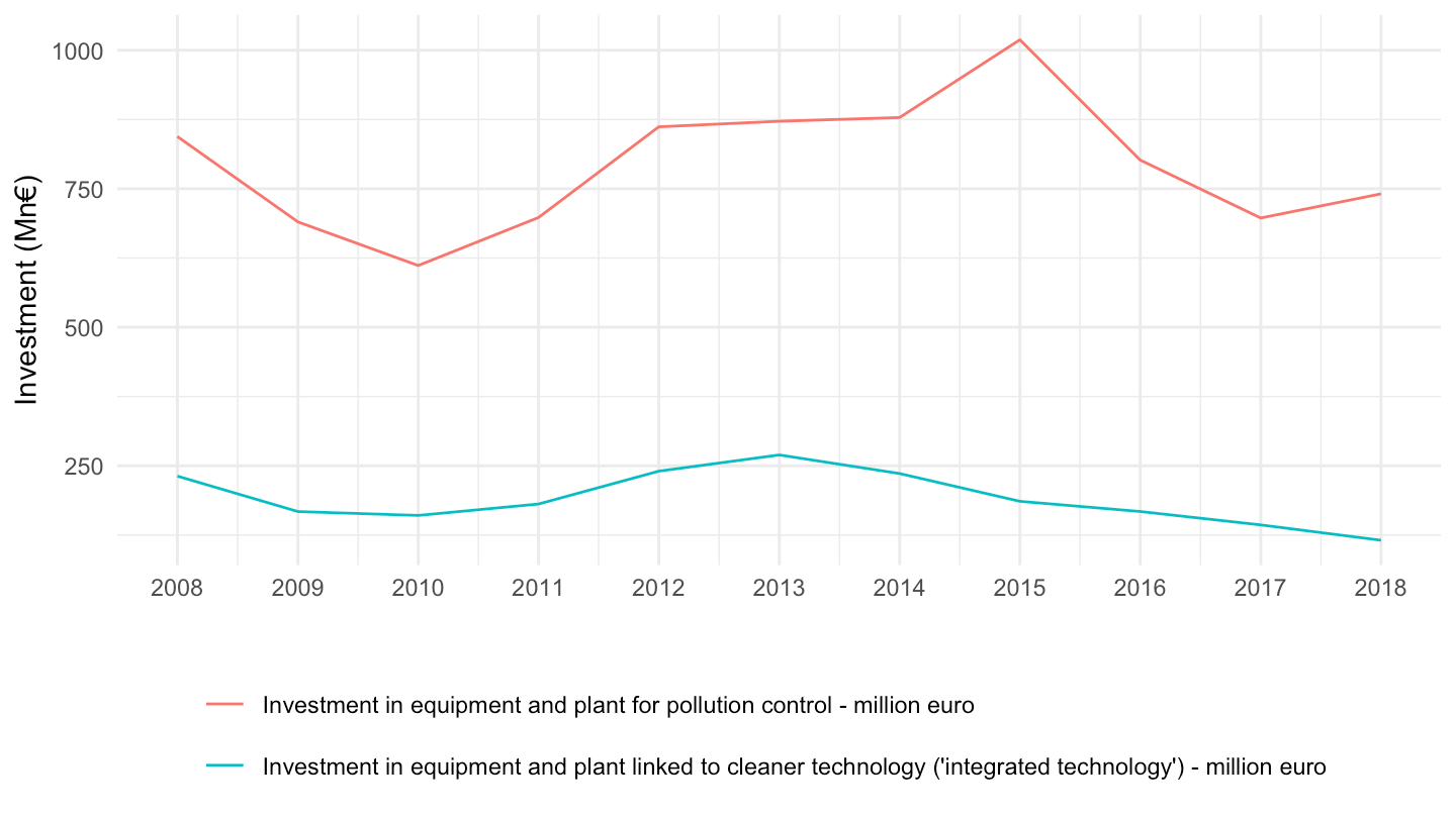

Latest Year, Manufacturing (Mn€)

Code

latest_y_sbs <- sbs_env_sc_r2 |>
  filter(nace_r2 == "C",
         size_emp == "TOTAL",
         indic_sb == "V21110",
         geo %in% c("FR", "DE", "IT", "ES"),
         !is.na(values)) |>
  summarise(m = max(time)) |>
  pull(m)

sbs_env_sc_r2 |>
  filter(geo %in% c("FR", "DE", "IT", "ES"),
         nace_r2 == "C",
         size_emp == "TOTAL",
         time == latest_y_sbs) |>
  select(indic_sb, Indic_sb, Geo, values) |>
  spread(Geo, values) |>
  print_table_conditional()

indic_sb	Indic_sb	France	Germany	Italy	Spain
V21110	Investment in equipment and plant for pollution control - million euro	740.8	838.5	355.1	116.3
V21120	Investment in equipment and plant linked to cleaner technology ('integrated technology') - million euro	115.6	749.0	157.6	382.4