| source | dataset | Title | Download | Compile |
|---|---|---|---|---|
| ec | WOB | Weekly Oil Bulletin | 2024-08-25 | [2026-01-16] |
| eurostat | ei_isen_m | Energy - monthly data | 2026-03-23 | [2026-03-24] |
| eurostat | nrg_bal_c | Complete energy balances | 2026-03-23 | [2023-12-31] |
| eurostat | nrg_pc_202 | Gas prices for household consumers - bi-annual data (from 2007 onwards) | 2026-03-23 | [2026-03-22] |
| eurostat | nrg_pc_203 | Gas prices for non-household consumers - bi-annual data (from 2007 onwards) | 2026-03-23 | [2023-06-11] |
| eurostat | nrg_pc_203_c | Gas prices components for non-household consumers - annual data | 2026-03-23 | [2026-03-22] |
| eurostat | nrg_pc_203_h | Gas prices for industrial consumers - bi-annual data (until 2007) | 2026-03-23 | [2026-03-22] |
| eurostat | nrg_pc_203_v | Non-household consumption volumes of gas by consumption bands | 2026-03-23 | [2026-03-22] |
| eurostat | nrg_pc_204 | Electricity prices for household consumers - bi-annual data (from 2007 onwards) | 2026-03-23 | [2026-03-22] |
| eurostat | nrg_pc_205 | Electricity prices for non-household consumers - bi-annual data (from 2007 onwards) | 2026-03-23 | [2023-06-11] |
| fred | energy | Energy | 2026-03-23 | [2026-03-23] |
| iea | world_energy_balances_highlights_2022 | World Energy Balances Highlights (2022 edition) | 2023-04-24 | [2024-06-20] |
| wb | CMO | World Bank Commodity Price Data (The Pink Sheet) | 2026-01-07 | [2026-02-12] |
| wdi | EG.GDP.PUSE.KO.PP.KD | GDP per unit of energy use (constant 2017 PPP $ per kg of oil equivalent) | 2026-03-23 | [2026-03-23] |
| wdi | EG.USE.PCAP.KG.OE | Energy use (kg of oil equivalent per capita) | 2026-03-23 | [2026-03-23] |
| yahoo | energy | Energy | 2026-03-23 | [2026-03-23] |
Household consumption volumes of gas by consumption bands
Data - Eurostat
Info
LAST_COMPILE
| LAST_COMPILE |
|---|
| 2026-03-24 |
Last
Code
nrg_pc_202_v %>%
  group_by(time) %>%
  summarise(Nobs = n()) %>%
  arrange(desc(time)) %>%
  head(1) %>%
print_table_conditional()| time | Nobs |
|---|---|
| 2024 | 92 |
Info
Code
include_graphics("https://ec.europa.eu/eurostat/documents/4187653/14185664/Gas+and+Electricity+Prices+S1_2022.png")
nrg_cons
Code
nrg_pc_202_v %>%
  left_join(nrg_cons, by = "nrg_cons") %>%
  group_by(nrg_cons, Nrg_cons) %>%
  summarise(Nobs = n()) %>%
  arrange(-Nobs) %>%
print_table_conditional()| nrg_cons | Nrg_cons | Nobs |
|---|---|---|
| GJ20-199 | Consumption from 20 GJ to 199 GJ - band D2 | 256 |
| GJ_LT20 | Consumption less than 20 GJ - band D1 | 256 |
| GJ_GE200 | Consumption 200 GJ or over - band D3 | 243 |
geo
Code
nrg_pc_202_v %>%
  left_join(geo, by = "geo") %>%
  group_by(geo, Geo) %>%
  summarise(Nobs = n()) %>%
  arrange(-Nobs) %>%
  mutate(Geo = ifelse(geo == "DE", "Germany", Geo)) %>%
  mutate(Flag = gsub(" ", "-", str_to_lower(Geo)),
         Flag = paste0('<img src="../../bib/flags/vsmall/', Flag, '.png" alt="Flag">')) %>%
  select(Flag, everything()) %>%
  {if (is_html_output()) datatable(., filter = 'top', rownames = F, escape = F) else .}
time
Code
nrg_pc_202_v %>%
  group_by(time) %>%
  summarise(Nobs = n()) %>%
  arrange(desc(time)) %>%
print_table_conditional()| time | Nobs |
|---|---|
| 2024 | 92 |
| 2023 | 91 |
| 2022 | 95 |
| 2021 | 94 |
| 2020 | 97 |
| 2019 | 101 |
| 2018 | 97 |
| 2017 | 88 |
Example
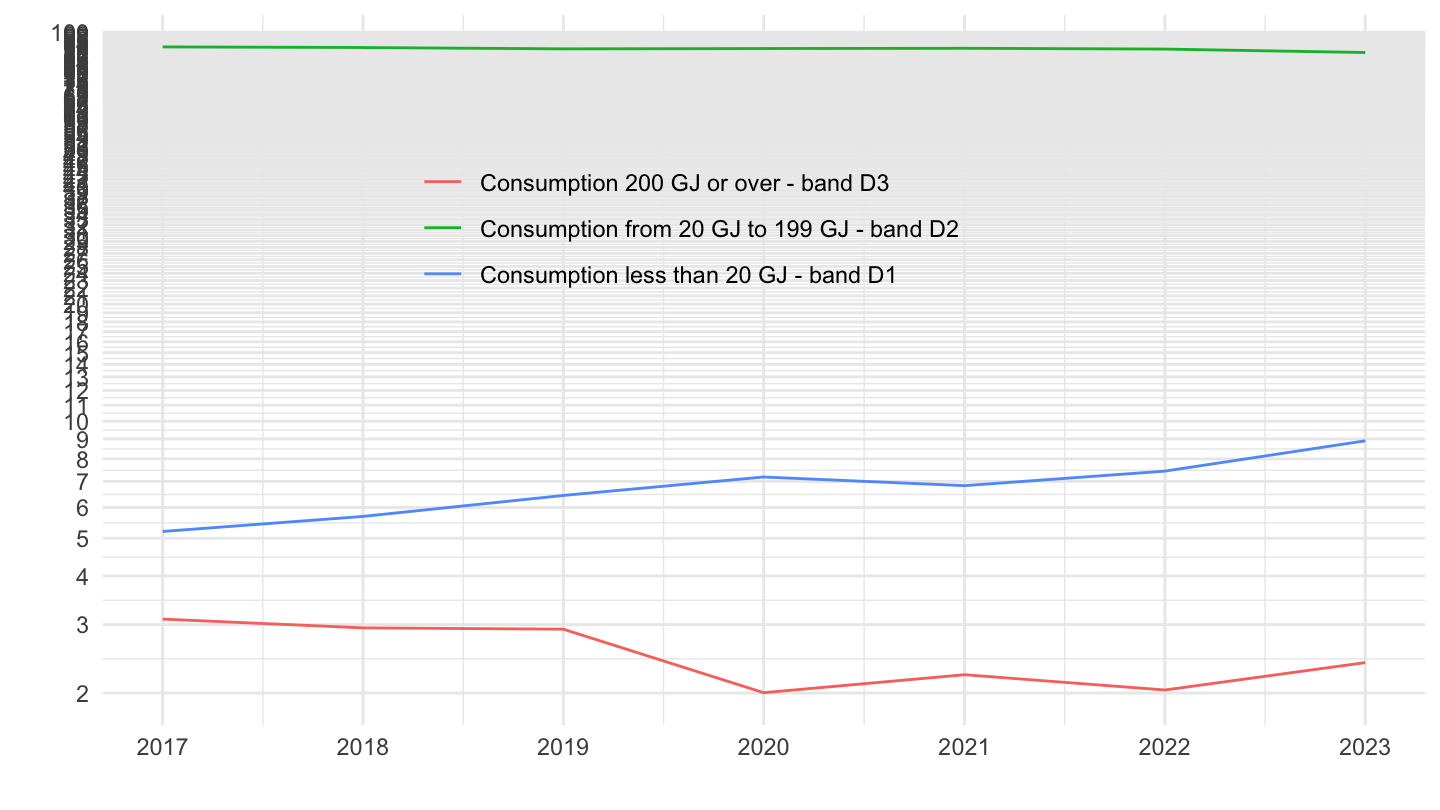
France
Code
nrg_pc_202_v %>%
  filter(geo == "FR") %>%
  left_join(nrg_cons, by = "nrg_cons") %>%
  select_if(~ n_distinct(.) > 1) %>%
  year_to_date %>%
  ggplot + geom_line(aes(x = date, y = values, color = Nrg_cons)) +
  theme_minimal() + xlab("") + ylab("") +
  scale_x_date(breaks = seq(1920, 2025, 1) %>% paste0("-01-01") %>% as.Date,
               labels = date_format("%Y")) +
  scale_y_log10(breaks = seq(1, 100, 1)) +
  theme(legend.position = c(0.45, 0.7),
        legend.title = element_blank())
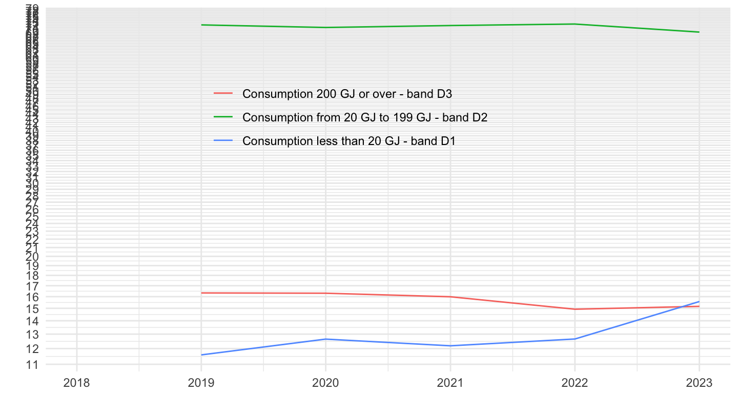
Germany
Code
nrg_pc_202_v %>%
  filter(geo == "DE") %>%
  left_join(nrg_cons, by = "nrg_cons") %>%
  select_if(~ n_distinct(.) > 1) %>%
  year_to_date %>%
  ggplot + geom_line(aes(x = date, y = values, color = Nrg_cons)) +
  theme_minimal() + xlab("") + ylab("") +
  scale_x_date(breaks = seq(1920, 2025, 1) %>% paste0("-01-01") %>% as.Date,
               labels = date_format("%Y")) +
  scale_y_log10(breaks = seq(1, 100, 1)) +
  theme(legend.position = c(0.45, 0.7),
        legend.title = element_blank())
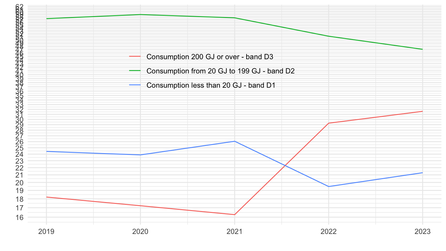
Italy
Code
nrg_pc_202_v %>%
  filter(geo == "IT") %>%
  left_join(nrg_cons, by = "nrg_cons") %>%
  select_if(~ n_distinct(.) > 1) %>%
  year_to_date %>%
  ggplot + geom_line(aes(x = date, y = values, color = Nrg_cons)) +
  theme_minimal() + xlab("") + ylab("") +
  scale_x_date(breaks = seq(1920, 2025, 1) %>% paste0("-01-01") %>% as.Date,
               labels = date_format("%Y")) +
  scale_y_log10(breaks = seq(1, 100, 1)) +
  theme(legend.position = c(0.45, 0.7),
        legend.title = element_blank())
Spain
Code
nrg_pc_202_v %>%
  filter(geo == "ES") %>%
  left_join(nrg_cons, by = "nrg_cons") %>%
  select_if(~ n_distinct(.) > 1) %>%
  year_to_date %>%
  ggplot + geom_line(aes(x = date, y = values, color = Nrg_cons)) +
  theme_minimal() + xlab("") + ylab("") +
  scale_x_date(breaks = seq(1920, 2025, 1) %>% paste0("-01-01") %>% as.Date,
               labels = date_format("%Y")) +
  scale_y_log10(breaks = seq(1, 100, 1)) +
  theme(legend.position = c(0.45, 0.7),
        legend.title = element_blank())