Final consumption aggregates - namq_10_fcs

Data - Eurostat

Author

François Geerolf

Info

Last observation: Quarterly: 2026Q1 (N = 8,453)

First observation: Quarterly: 1978Q1 (N = 180)

Last data update: 23 jul 2026, 23:00. Last compile: 24 jul 2026, 03:00

Structure

France

Table

Code

namq_10_fcs %>%
  filter(geo == "FR",
         time == "2021Q4",
         s_adj == "NSA") %>%
  select_if(~ n_distinct(.) > 1) %>%
  
  
  mutate(Na_item = paste0(na_item, " - ", Na_item)) %>%
  select(-na_item) %>%
  spread(Na_item, values) %>%
  print_table_conditional()

unit	Unit	P31_S14 - Final consumption expenditure of household	P311_S14 - Final consumption expenditure of households, durable goods	P312_S14 - Final consumption expenditure of households, semi-durable goods	P312N_S14 - Final consumption expenditure of households, semi-durable goods, non-durable goods and services	P313_S14 - Final consumption expenditure of households, non-durable goods	P314_S14 - Final consumption expenditure of households, services
CLV_I05	Chain linked volumes, index 2005=100	122.531	145.406	115.906	120.468	111.916	126.214
CLV_I10	Chain linked volumes, index 2010=100	114.000	121.197	113.834	113.398	107.427	116.671
CLV_I15	Chain linked volumes, index 2015=100	109.875	118.800	112.418	109.105	106.627	109.834
CLV_I20	Chain linked volumes, index 2020=100	111.821	112.026	117.573	111.803	108.096	113.002
CLV_PCH_SM	Chain linked volumes, percentage change compared to same period in previous year	7.500	-0.900	9.200	8.300	0.400	13.000
CLV05_MEUR	Chain linked volumes (2005), million euro	287416.500	32995.700	28427.400	255239.800	74952.800	151930.700
CLV05_MNAC	Chain linked volumes (2005), million units of national currency	287416.500	32995.700	28427.400	255239.800	74952.800	151930.700
CLV10_MEUR	Chain linked volumes (2010), million euro	305984.700	29206.900	28957.500	277041.600	82705.300	165534.800
CLV10_MNAC	Chain linked volumes (2010), million units of national currency	305984.700	29206.900	28957.500	277041.600	82705.300	165534.800
CLV15_MEUR	Chain linked volumes (2015), million euro	318545.500	27753.900	29625.100	290823.200	89106.900	172036.100
CLV15_MNAC	Chain linked volumes (2015), million units of national currency	318545.500	27753.900	29625.100	290823.200	89106.900	172036.100
CLV20_MEUR	Chain linked volumes (2020), million euro	332936.200	26854.100	29277.000	306082.100	97393.400	179411.700
CLV20_MNAC	Chain linked volumes (2020), million units of national currency	332936.200	26854.100	29277.000	306082.100	97393.400	179411.700
CP_MEUR	Current prices, million euro	340524.600	27763.400	30327.300	312761.200	100696.900	181737.000
CP_MNAC	Current prices, million units of national currency	340524.600	27763.400	30327.300	312761.200	100696.900	181737.000
PC_GDP	Percentage of gross domestic product (GDP)	51.500	4.200	4.600	47.300	15.200	27.500
PYP_MEUR	Previous year prices, million euro	332936.200	26854.100	29277.000	306082.100	97393.400	179411.700
PYP_MNAC	Previous year prices, million units of national currency	332936.200	26854.100	29277.000	306082.100	97393.400	179411.700

France, Germany, Spain, Italy, Netherlands

All

Consumption

Code

namq_10_fcs %>%
  filter(geo %in% c("FR", "EA", "ES", "IT", "DE"),
         unit == "PC_GDP",
         s_adj == "NSA",
         na_item == "P31_S14") %>%
  quarter_to_date %>%
  mutate(values = values / 100) %>%
  
  mutate(Geo = ifelse(geo == "EA", "Europe", Geo)) %>%
  left_join(colors, by = c("Geo" = "country")) %>%
  mutate(color = ifelse(geo == "EA", color2, color)) %>%
  ggplot + geom_line(aes(x = date, y = values, color = color)) +
  scale_color_identity() + theme_minimal()  + add_4flags + xlab("") + 
  ylab("Final consumption expenditure of households (% of GDP)") +
  scale_x_date(breaks = as.Date(paste0(seq(1960, 2100, 5), "-01-01")),
               labels = date_format("%Y")) +
  scale_y_continuous(breaks = 0.01*seq(-30, 100, 2),
                labels = percent_format(a = 1))

1995-

Consumption

Code

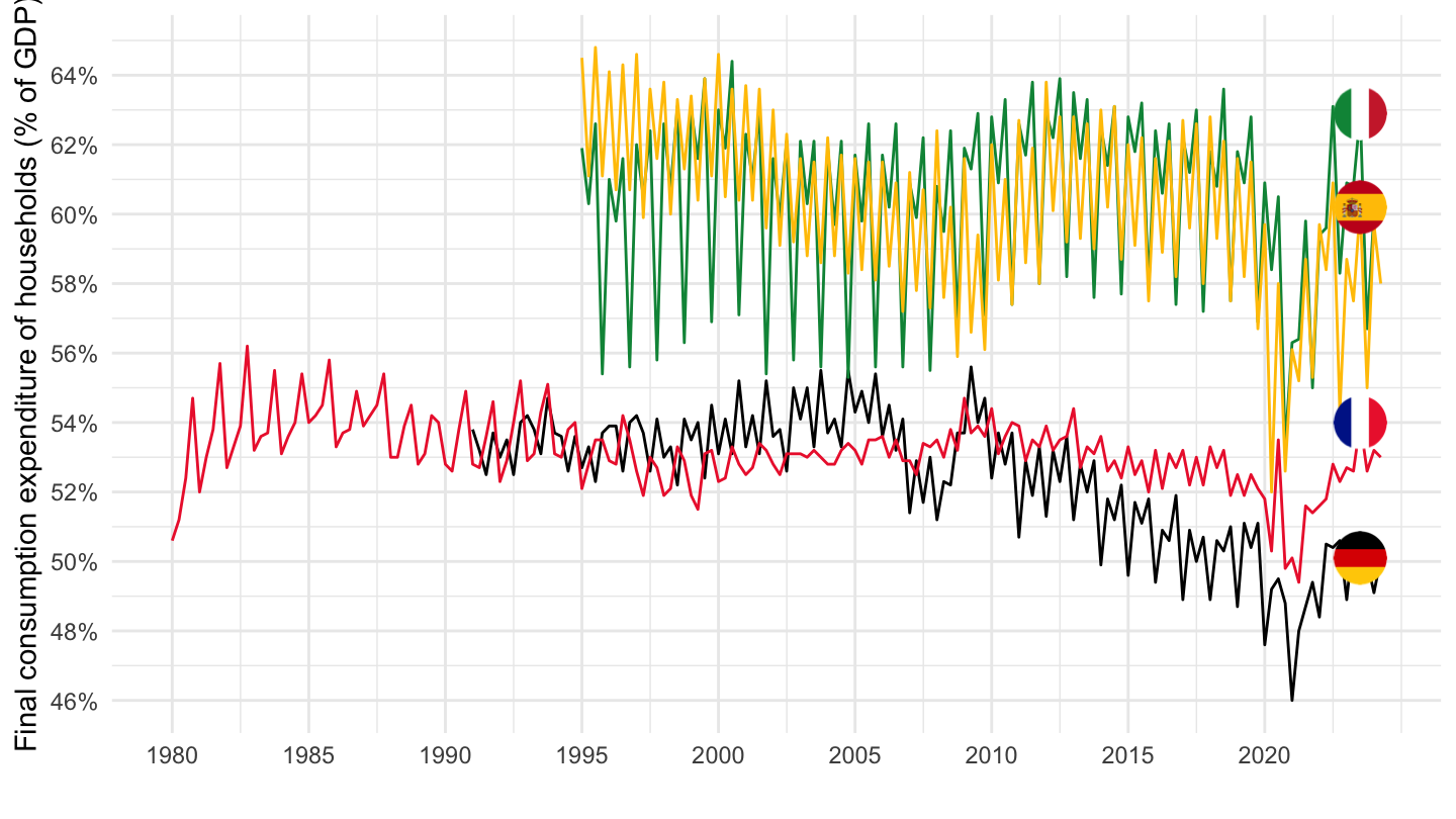
namq_10_fcs %>%
  filter(geo %in% c("FR", "NL", "ES", "IT", "DE"),
         unit == "PC_GDP",
         s_adj == "NSA",
         na_item == "P31_S14") %>%
  quarter_to_date %>%
  filter(date >= as.Date("1995-01-01")) %>%
  mutate(values = values / 100) %>%
  
  left_join(colors, by = c("Geo" = "country")) %>%
  mutate(color = ifelse(geo == "NL", color2, color)) %>%
  ggplot + geom_line(aes(x = date, y = values, color = color)) +
  scale_color_identity() + theme_minimal()  + add_4flags + xlab("") + 
  ylab("Final consumption expenditure of households (% of GDP)") +
  scale_x_date(breaks = as.Date(paste0(seq(1960, 2100, 5), "-01-01")),
               labels = date_format("%Y")) +
  scale_y_continuous(breaks = 0.01*seq(-30, 100, 2),
                labels = percent_format(a = 1))

Durable goods

Code

namq_10_fcs %>%
  filter(geo %in% c("FR", "NL", "ES", "IT", "DE"),
         unit == "PC_GDP",
         s_adj == "NSA",
         na_item == "P311_S14") %>%
  quarter_to_date %>%
  filter(date >= as.Date("1995-01-01")) %>%
  mutate(values = values / 100) %>%
  
  left_join(colors, by = c("Geo" = "country")) %>%
  mutate(color = ifelse(geo == "NL", color2, color)) %>%
  ggplot + geom_line(aes(x = date, y = values, color = color)) +
  scale_color_identity() + theme_minimal()  + add_4flags + xlab("") + 
  ylab("Durable goods (% of GDP)") +
  scale_x_date(breaks = as.Date(paste0(seq(1960, 2100, 5), "-01-01")),
               labels = date_format("%Y")) +
  scale_y_continuous(breaks = 0.01*seq(-30, 100, 1),
                labels = percent_format(a = 1))

Non-durable goods

Code

namq_10_fcs %>%
  filter(geo %in% c("FR", "NL", "ES", "IT", "DE"),
         unit == "PC_GDP",
         s_adj == "NSA",
         na_item == "P313_S14") %>%
  quarter_to_date %>%
  filter(date >= as.Date("1995-01-01")) %>%
  mutate(values = values / 100) %>%
  
  left_join(colors, by = c("Geo" = "country")) %>%
  mutate(color = ifelse(geo == "NL", color2, color)) %>%
  ggplot + geom_line(aes(x = date, y = values, color = color)) +
  scale_color_identity() + theme_minimal()  + add_4flags + xlab("") + 
  ylab("Non-durable goods (% of GDP)") +
  scale_x_date(breaks = as.Date(paste0(seq(1960, 2100, 5), "-01-01")),
               labels = date_format("%Y")) +
  scale_y_continuous(breaks = 0.01*seq(-30, 100, 1),
                labels = percent_format(a = 1))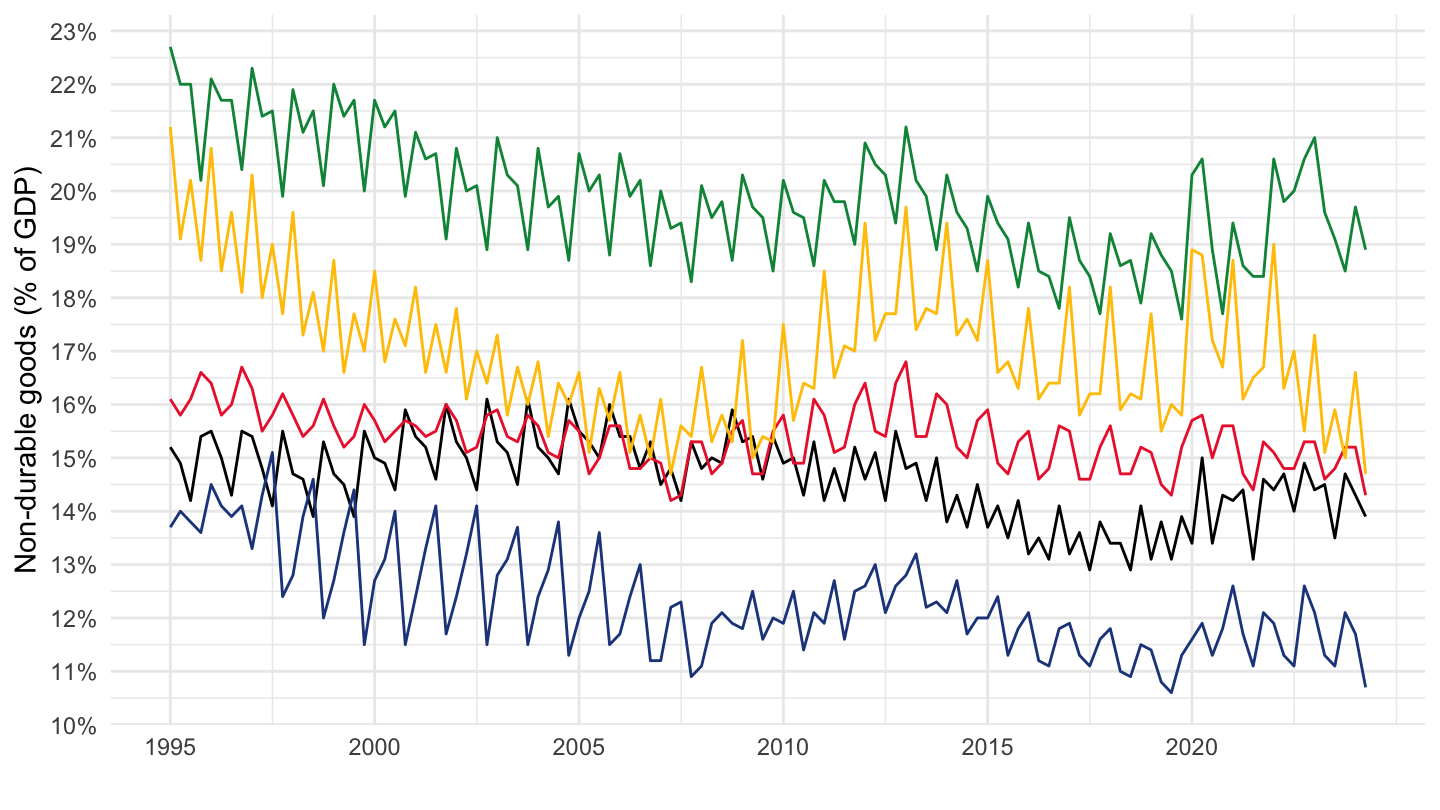

Services

Code

namq_10_fcs %>%
  filter(geo %in% c("FR", "NL", "ES", "IT", "DE"),
         unit == "PC_GDP",
         s_adj == "NSA",
         na_item == "P314_S14") %>%
  quarter_to_date %>%
  filter(date >= as.Date("1995-01-01")) %>%
  mutate(values = values / 100) %>%
  
  left_join(colors, by = c("Geo" = "country")) %>%
  mutate(color = ifelse(geo == "NL", color2, color)) %>%
  ggplot + geom_line(aes(x = date, y = values, color = color)) +
  scale_color_identity() + theme_minimal()  + add_4flags + xlab("") + 
  ylab("Services (% of GDP)") +
  scale_x_date(breaks = as.Date(paste0(seq(1960, 2100, 5), "-01-01")),
               labels = date_format("%Y")) +
  scale_y_continuous(breaks = 0.01*seq(-30, 100, 1),
                labels = percent_format(a = 1))