Gross domestic product (GDP) at current market prices by NUTS 3 regions - nama_10r_3gdp
Data - Eurostat
Info
Last observation: Annual: 2024 (N = 6,706)
First observation: Annual: 2000 (N = 11,556)
Last data update: 23 jul 2026, 22:37. Last compile: 24 jul 2026, 02:53
Structure
Table - Per Inhabitant
Code
nama_10r_3gdp %>%
  filter(time == "2017",
         unit %in% c("EUR_HAB", "PPS_EU27_2020_HAB")) %>%
  select(geo, unit, values) %>%

  spread(unit, values) %>%
  arrange(-`EUR_HAB`) %>%
  print_table_conditional()
NUTS 0
Code
nama_10r_3gdp %>%
  filter(time == "2016",
         nchar(geo) == 2,
         unit == "EUR_HAB") %>%
  right_join(europe_NUTS0, by = "geo") %>%
  filter(long >= -15, lat >= 33) %>%
  ggplot(., aes(x = long, y = lat, group = group, fill = values/1000)) +
  geom_polygon() + coord_map() +
  scale_fill_viridis_c(na.value = "white",
                       labels = scales::dollar_format(accuracy = 1, prefix = "", suffix = " k€"),
                       breaks = seq(0, 200, 10),
                       values = c(0, 0.1, 0.2, 0.3, 0.4, 0.5, 1)) +
  theme_void() + theme(legend.position = c(0.25, 0.85)) +
  labs(fill = "€ / inhabitant")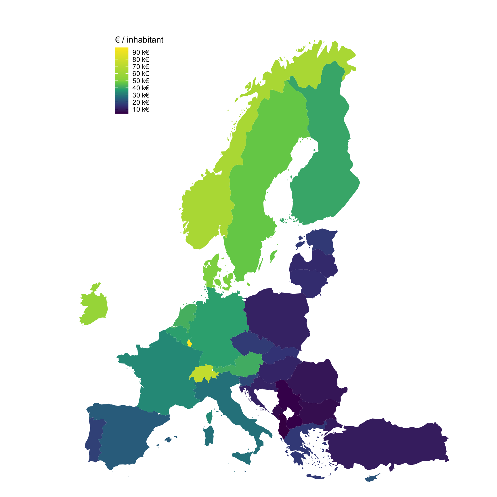
NUTS 1
EUR_HAB
Code
nama_10r_3gdp %>%
  filter(time == "2016",
         nchar(geo) == 3,
         unit == "EUR_HAB") %>%
  right_join(europe_NUTS1, by = "geo") %>%
  filter(long >= -15, lat >= 33) %>%
  ggplot(., aes(x = long, y = lat, group = group, fill = values/1000)) +
  geom_polygon() + coord_map() +
  scale_fill_viridis_c(na.value = "white",
                       labels = scales::dollar_format(accuracy = 1, prefix = "", suffix = " k€"),
                       breaks = seq(0, 200, 10),
                       values = c(0, 0.1, 0.2, 0.3, 0.4, 0.5, 1)) +
  theme_void() + theme(legend.position = c(0.25, 0.85)) +
  labs(fill = "€ / inhabitant")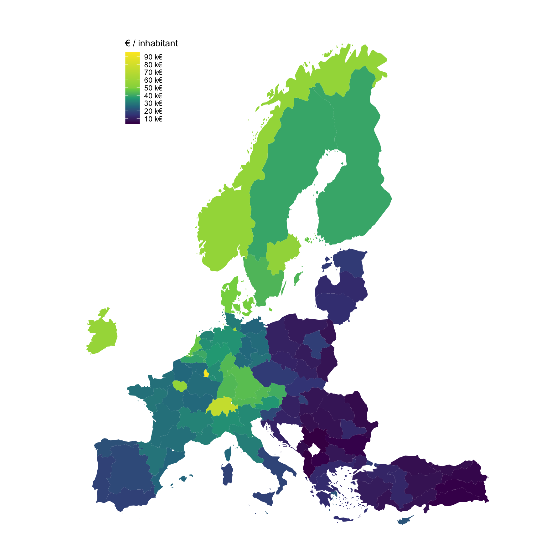
PPS_EU27_2020_HAB
Code
nama_10r_3gdp %>%
  filter(time == "2016",
         nchar(geo) == 3,
         unit == "PPS_EU27_2020_HAB") %>%
  right_join(europe_NUTS1, by = "geo") %>%
  filter(long >= -15, lat >= 33) %>%
  ggplot(., aes(x = long, y = lat, group = group, fill = values/1000)) +
  geom_polygon() + coord_map() +
  scale_fill_viridis_c(na.value = "white",
                       labels = scales::dollar_format(accuracy = 1, prefix = "", suffix = " k€"),
                       breaks = seq(0, 200, 10),
                       values = c(0, 0.1, 0.2, 0.3, 0.4, 0.5, 1)) +
  theme_void() + theme(legend.position = c(0.25, 0.85)) +
  labs(fill = "€ / inhabitant")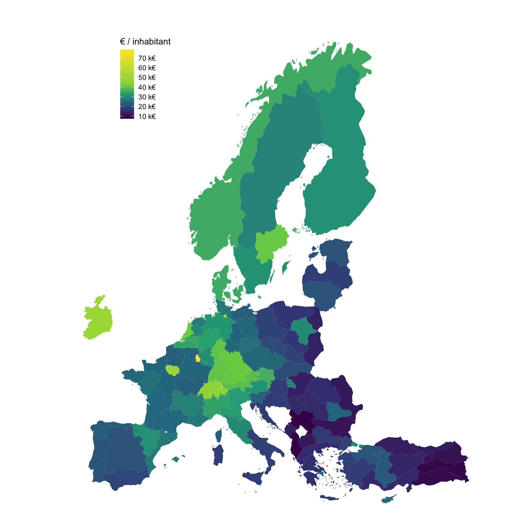
NUTS 2
EUR_HAB
Code
nama_10r_3gdp %>%
  filter(time == "2016",
         nchar(geo) == 4,
         unit == "EUR_HAB") %>%
  right_join(europe_NUTS2, by = "geo") %>%
  filter(long >= -15, lat >= 33) %>%
  ggplot(., aes(x = long, y = lat, group = group, fill = values/1000)) +
  geom_polygon() + coord_map() +
  scale_fill_viridis_c(na.value = "white",
                       labels = scales::dollar_format(accuracy = 1, prefix = "", suffix = " k€"),
                       breaks = seq(0, 200, 20),
                       values = c(0, 0.05, 0.1, 0.15, 0.2, 0.25, 1)) +
  theme_void() + theme(legend.position = c(0.25, 0.85)) +
  labs(fill = "€ / inhabitant")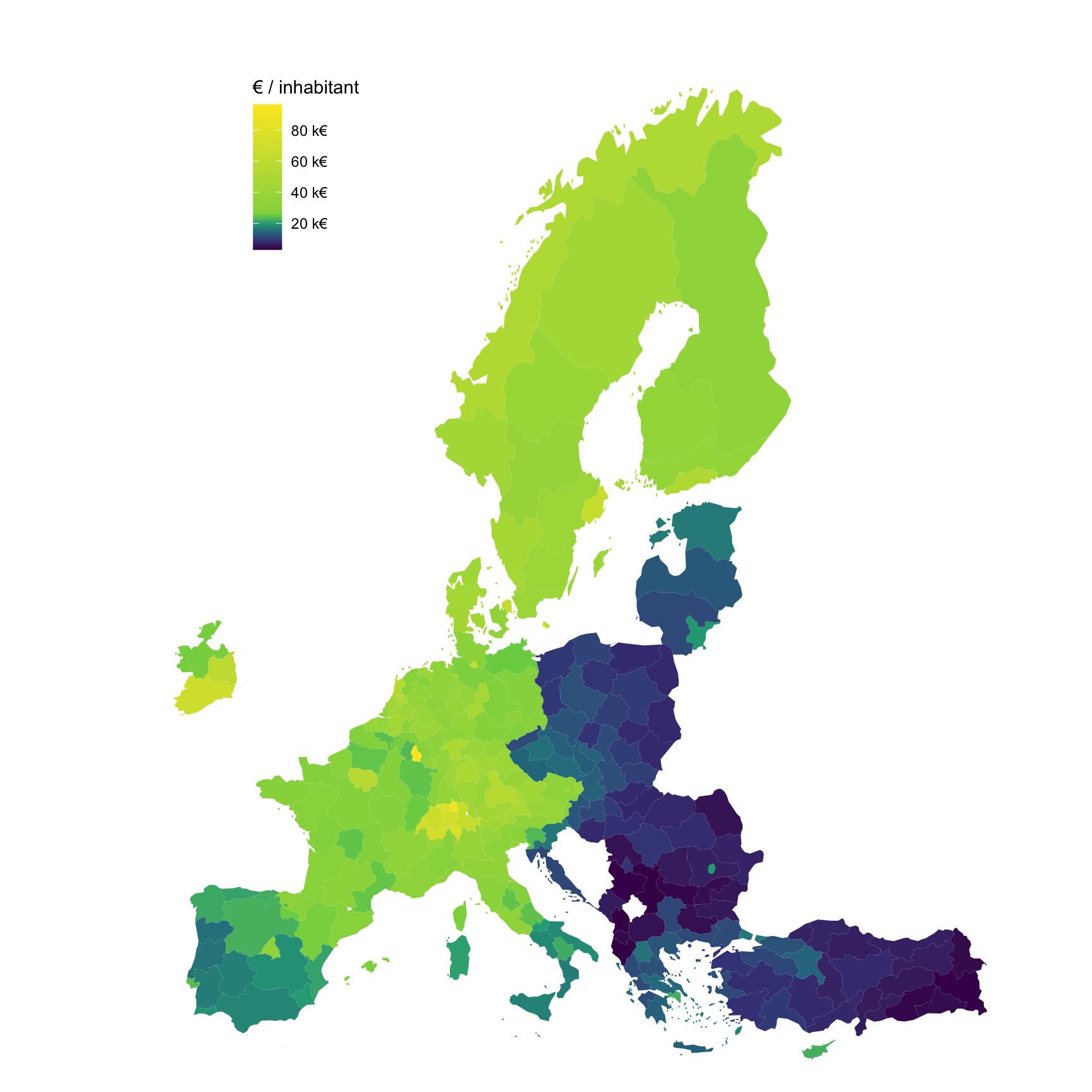
PPS_EU27_2020_HAB
Code
nama_10r_3gdp %>%
  filter(time == "2016",
         nchar(geo) == 4,
         unit == "PPS_EU27_2020_HAB") %>%
  right_join(europe_NUTS2, by = "geo") %>%
  filter(long >= -15, lat >= 33) %>%
  ggplot(., aes(x = long, y = lat, group = group, fill = values/1000)) +
  geom_polygon() + coord_map() +
  scale_fill_viridis_c(na.value = "white",
                       labels = scales::dollar_format(accuracy = 1, prefix = "", suffix = " k€"),
                       breaks = seq(0, 200, 20),
                       values = c(0, 0.05, 0.1, 0.15, 0.2, 0.25, 1)) +
  theme_void() + theme(legend.position = c(0.25, 0.85)) +
  labs(fill = "€ / inhabitant")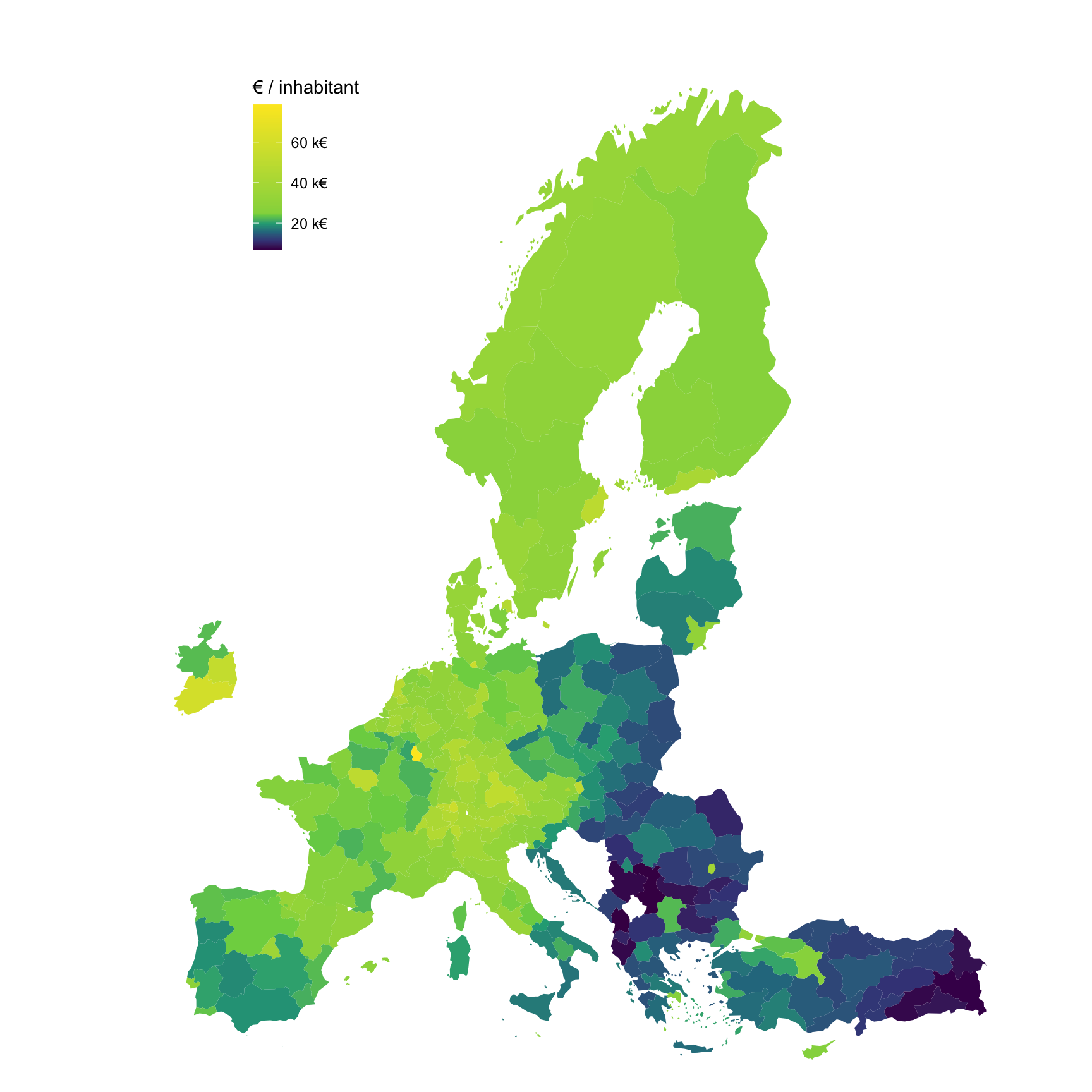
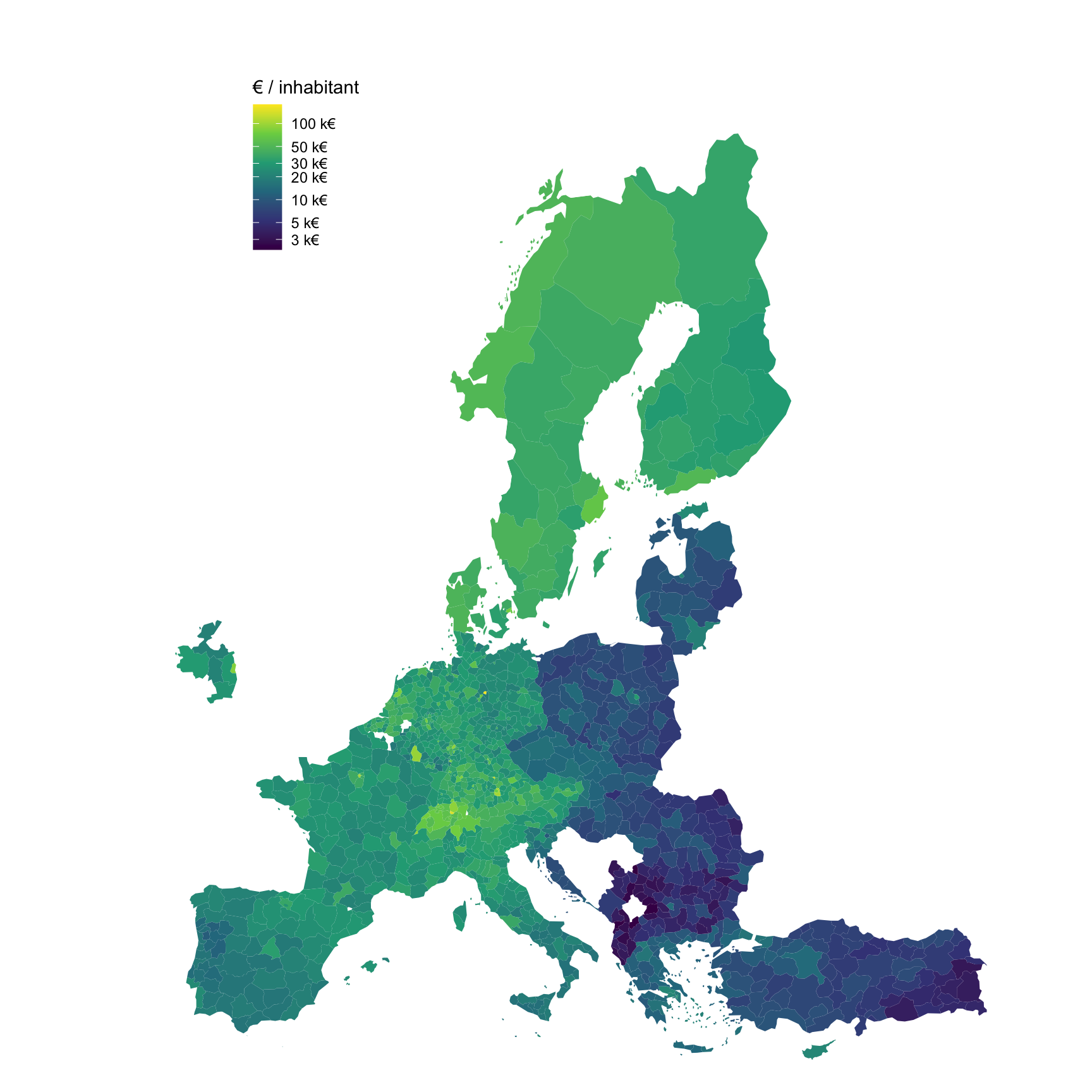
NUTS 3
2016
Code
nama_10r_3gdp %>%
  filter(time == "2016",
         nchar(geo) == 5,
         unit == "EUR_HAB") %>%
  right_join(europe_NUTS3, by = "geo") %>%
  filter(long >= -15, lat >= 33) %>%
  ggplot(., aes(x = long, y = lat, group = group, fill = values/1000)) +
  geom_polygon() + coord_map() +
  scale_fill_viridis_c(na.value = "white",
                       labels = scales::dollar_format(accuracy = 1, prefix = "", suffix = " k€"),
                       breaks = seq(0, 600, 50),
                       values = c(0, 0.02, 0.04, 0.06, 0.08, 0.1, 1)) +
  theme_void() + theme(legend.position = c(0.25, 0.85)) +
  labs(fill = "€ / inhabitant")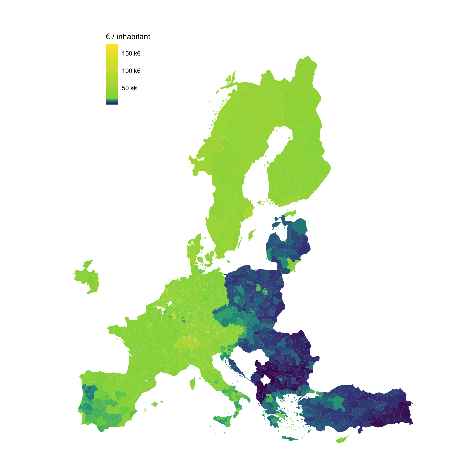
2019
Code
nama_10r_3gdp %>%
  filter(time == "2019",
         nchar(geo) == 5,
         unit == "EUR_HAB") %>%
  right_join(europe_NUTS3, by = "geo") %>%
  filter(long >= -15, lat >= 33) %>%
  ggplot(., aes(x = long, y = lat, group = group, fill = values/1000)) +
  geom_polygon() + coord_map() +
  scale_fill_viridis_c(na.value = "white",
                       labels = scales::dollar_format(accuracy = 1, prefix = "", suffix = " k€"),
                       breaks = seq(10, 250, 30),
                       values = c(0, 0.1, 0.15, 0.2, 0.25, 0.3,0.35, 1)) +
  theme_void() + theme(legend.position = c(0.25, 0.85)) +
  labs(fill = "PIB / habitant, 2019\n(milliers €)\n")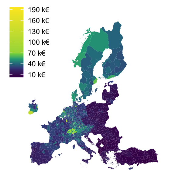
2018
Code
nama_10r_3gdp %>%
  filter(time == "2018",
         nchar(geo) == 5,
         unit == "EUR_HAB") %>%
  right_join(europe_NUTS3, by = "geo") %>%
  filter(long >= -15, lat >= 33) %>%
  ggplot(., aes(x = long, y = lat, group = group, fill = values/1000)) +
  geom_polygon() + coord_map() +
  scale_fill_viridis_c(na.value = "white",
                       labels = scales::dollar_format(accuracy = 1, prefix = "", suffix = " k€"),
                       breaks = seq(10, 250, 30),
                       values = c(0, 0.1, 0.15, 0.2, 0.25, 0.3, 0.35, 0.4, 0.45, 1)) +
  theme_void() + theme(legend.position = c(0.25, 0.85)) +
  labs(fill = "PIB / habitant\n(milliers €)\n")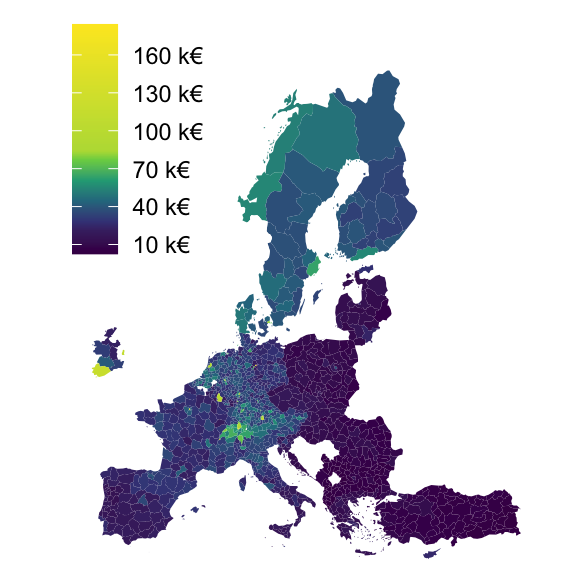
NUTS 3 - Log
Code
nama_10r_3gdp %>%
  filter(time == "2016",
         nchar(geo) == 5,
         unit == "EUR_HAB") %>%
  right_join(europe_NUTS3, by = "geo") %>%
  filter(long >= -15, lat >= 33) %>%
  ggplot(., aes(x = long, y = lat, group = group, fill = values/1000)) +
  geom_polygon() + coord_map() +
  scale_fill_viridis_c(na.value = "white",
                       labels = scales::dollar_format(accuracy = 1, prefix = "", suffix = " k€"),
                       breaks = c(1, 2, 3, 5, 10, 20, 30, 50, 100, 200, 300, 1000),
                       trans = scales::pseudo_log_trans(sigma = 0.001)) +
  theme_void() + theme(legend.position = c(0.25, 0.85)) +
  labs(fill = "€ / inhabitant")