Top 20 ports - gross weight of goods handled in each port, by type of cargo (main ports)
Data - Eurostat
Info
Last observation: Annual: 2024 (N = 398)
First observation: Annual: 2005 (N = 410)
Last data update: 23 jul 2026, 22:33. Last compile: 24 jul 2026, 02:33
Structure
Top 20 Ports
Ports of the Europe by annual cargo tonnage
Code
i_g("bib/industrie/top-20-ports.png")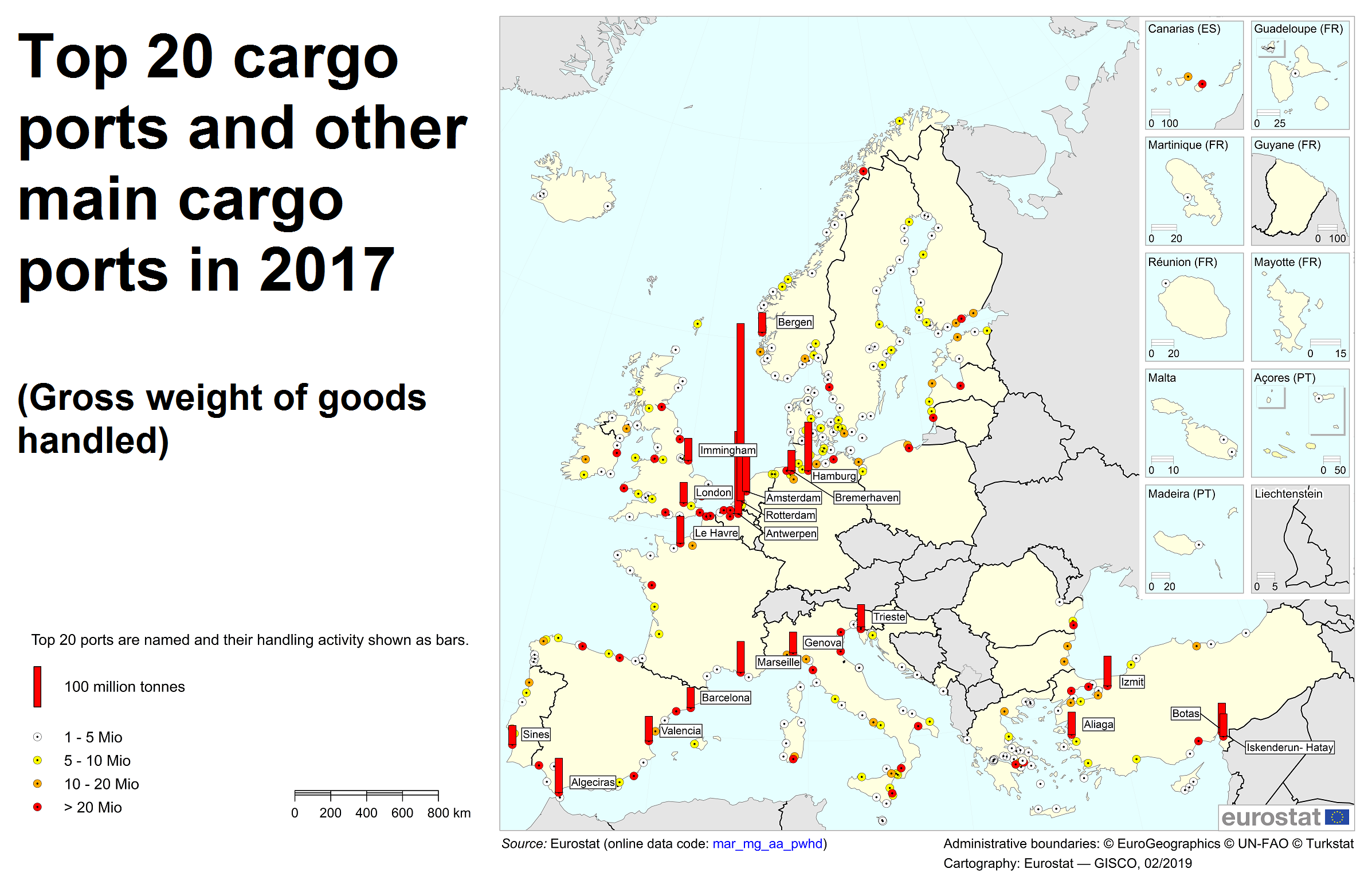
Conteneurs
2019
Code
mar_mg_am_pwhc %>%
  filter(unit == "THS_T",
         time == "2019",
         cargo == "TOTAL") %>%

  select(rep_mar, Rep_mar, values) %>%
  arrange(-values) %>%
  {if (is_html_output()) datatable(., filter = 'top', rownames = F, escape = F) else .}
2020
Code
mar_mg_am_pwhc %>%
  filter(unit == "THS_T",
         time == "2020",
         cargo == "TOTAL") %>%

  select(rep_mar, Rep_mar, values) %>%
  arrange(-values) %>%
  {if (is_html_output()) datatable(., filter = 'top', rownames = F, escape = F) else .}
Marseille, Antwerpen, Hamburg, Rotterdam
Code
mar_mg_am_pwhc %>%

  filter(cargo == "TOTAL",
         unit == "THS_T",
         Rep_mar %in% c("Rotterdam", "Antwerpen", "Hamburg", "Marseille")) %>%
  year_to_date %>%
  ggplot + geom_line(aes(x = date, y = values, color = Rep_mar)) +
     theme_minimal() + xlab("") + ylab("Volumes des conteneurs (Millions EVP)") +

  theme(legend.position = c(0.3, 0.85),
        legend.title = element_blank()) +
  scale_x_date(breaks = seq(1940, 2100, 2) %>% paste0("-01-01") %>% as.Date,
               labels = date_format("%Y")) +
  scale_y_continuous(breaks = seq(0, 20, 1))
FR_2FRMRS
Antwerpen, Hamburg, Rotterdam
Code
mar_mg_am_pwhc %>%

  filter(cargo == "TOTAL",
         unit == "THS_T",
         Rep_mar %in% c("Rotterdam", "Antwerpen", "Hamburg")) %>%
  year_to_date %>%
  mutate(values = values / 10^3) %>%
  ggplot + geom_line(aes(x = date, y = values, color = Rep_mar)) +
     theme_minimal() + xlab("") + ylab("Volumes des conteneurs (Millions EVP)") +

  theme(legend.position = c(0.3, 0.85),
        legend.title = element_blank()) +
  scale_x_date(breaks = seq(1940, 2100, 2) %>% paste0("-01-01") %>% as.Date,
               labels = date_format("%Y")) +
  scale_y_continuous(breaks = seq(0, 20, 1))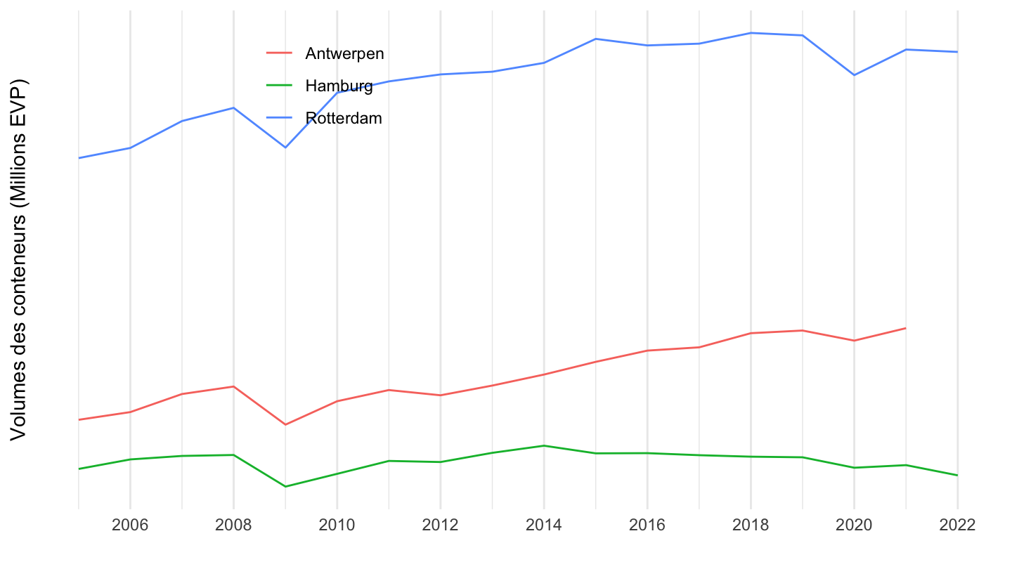
Peiraias, Valencia, Algeciras
Code
mar_mg_am_pwhc %>%

  filter(cargo == "TOTAL",
         unit == "THS_T",
         Rep_mar %in% c("Peiraias", "Valencia", "Algeciras")) %>%
  year_to_date %>%
  mutate(values = values / 10^3) %>%
  ggplot + geom_line(aes(x = date, y = values, color = Rep_mar)) +
     theme_minimal() + xlab("") + ylab("Volumes des conteneurs (Millions EVP)") +

  theme(legend.position = c(0.3, 0.85),
        legend.title = element_blank()) +
  scale_x_date(breaks = seq(1940, 2100, 2) %>% paste0("-01-01") %>% as.Date,
               labels = date_format("%Y")) +
  scale_y_continuous(breaks = seq(0, 20, 1))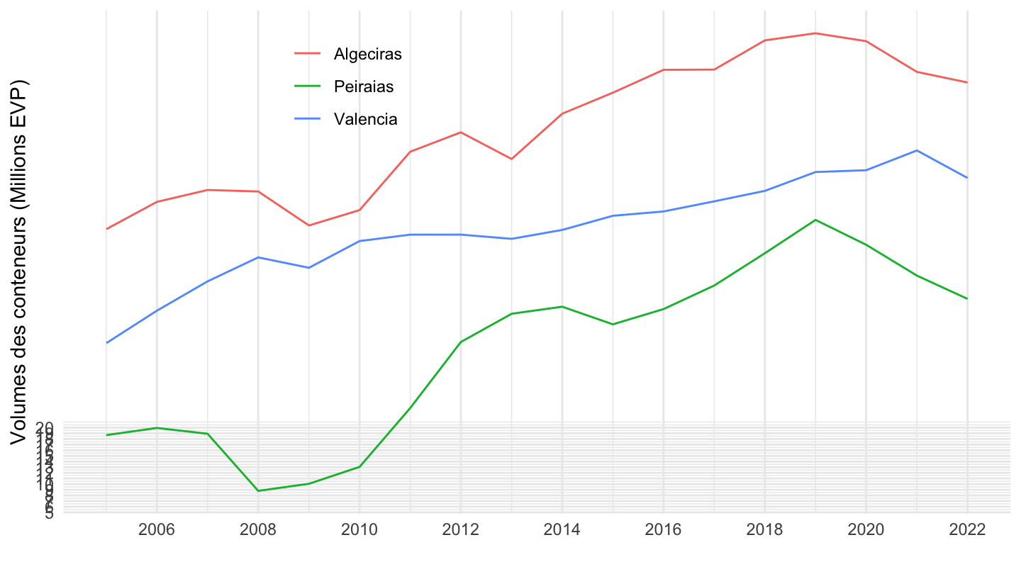
Bremerhaven, Felixstowe, Barcelona
Code
mar_mg_am_pwhc %>%

  filter(cargo == "TOTAL",
         unit == "THS_T",
         Rep_mar %in% c("Bremerhaven", "Felixstowe", "Barcelona")) %>%
  year_to_date %>%
  mutate(values = values / 10^3) %>%
  ggplot + geom_line(aes(x = date, y = values, color = Rep_mar)) +
     theme_minimal() + xlab("") + ylab("Volumes des conteneurs (Millions EVP)") +

  theme(legend.position = c(0.1, 0.85),
        legend.title = element_blank()) +
  scale_x_date(breaks = seq(1940, 2100, 2) %>% paste0("-01-01") %>% as.Date,
               labels = date_format("%Y")) +
  scale_y_continuous(breaks = seq(0, 20, 1))
Ambarli, Gioia Tauro, Le Havre
Code
mar_mg_am_pwhc %>%

  filter(cargo == "TOTAL",
         unit == "THS_T",
         Rep_mar %in% c("Ambarli", "Gioia Tauro", "Le Havre")) %>%
  year_to_date %>%
  mutate(values = values / 10^3) %>%
  ggplot + geom_line(aes(x = date, y = values, color = Rep_mar)) +
     theme_minimal() + xlab("") + ylab("Volumes des conteneurs (Millions EVP)") +

  theme(legend.position = c(0.1, 0.85),
        legend.title = element_blank()) +
  scale_x_date(breaks = seq(1940, 2100, 2) %>% paste0("-01-01") %>% as.Date,
               labels = date_format("%Y")) +
  scale_y_continuous(breaks = seq(0, 20, .5))
All ports
Linear
Code
mar_mg_am_pwhc %>%

  filter(cargo == "TOTAL",
         unit == "THS_T") %>%
  year_to_date %>%
  mutate(values = values / 10^3) %>%
  group_by(Rep_mar) %>%
  arrange(date) %>%
  mutate(values = 100*values/values[1]) %>%
  ggplot + geom_line(aes(x = date, y = values, color = Rep_mar)) +
  theme_minimal() + xlab("") + ylab("Volumes des conteneurs (Millions EVP)") +
  #scale_color_manual(values = viridis(13)[1:12]) +
  theme(legend.title = element_blank()) +
  scale_x_date(breaks = seq(1940, 2100, 5) %>% paste0("-01-01") %>% as.Date,
               labels = date_format("%Y")) +
  scale_y_log10(breaks = seq(10, 300, 10))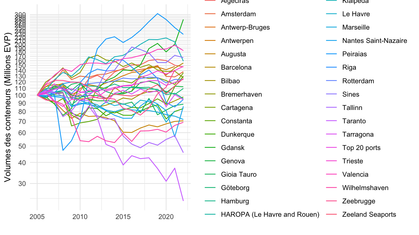
Largest
Code
mar_mg_am_pwhc %>%

  filter(cargo == "TOTAL",
         unit == "THS_T") %>%
  year_to_date %>%
  mutate(values = values / 10^3) %>%
  group_by(Rep_mar) %>%
  filter(n() == 18) %>%
  arrange(date) %>%
  filter(values[date == as.Date("2022-01-01")] > 40) %>%
  mutate(values = 100*values/values[1]) %>%
  ggplot + geom_line(aes(x = date, y = values, color = Rep_mar)) +
  theme_minimal() + xlab("") + ylab("Gross weight of goods handled in each port vs. 2005") +
  #scale_color_manual(values = viridis(13)[1:12]) +
  theme(legend.title = element_blank()) +
  scale_x_date(breaks = seq(1940, 2100, 2) %>% paste0("-01-01") %>% as.Date,
               labels = date_format("%Y")) +
  scale_y_log10(breaks = seq(10, 300, 10),
                labels = percent(0.01*seq(10, 300, 10)-1, 2)) +
  geom_text_repel(data = . %>% filter(date ==as.Date("2022-01-01")), aes(x = date, y = values, label = Rep_mar, color = Rep_mar))
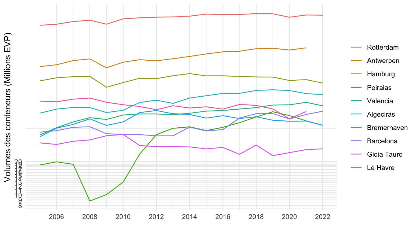
12 ports
Linear
Code
mar_mg_am_pwhc %>%

  filter(cargo == "TOTAL",
         unit == "THS_T",
         Rep_mar %in% c("Rotterdam", "Antwerpen", "Hamburg",
                        "Peiraias", "Valencia", "Algeciras",
                        "Bremerhaven", "Felixstowe", "Barcelona",
                        "Ambarli", "Gioia Tauro", "Le Havre")) %>%
  year_to_date %>%
  mutate(values = values / 10^3) %>%
  mutate(Rep_mar = factor(Rep_mar, c("Rotterdam", "Antwerpen", "Hamburg",
                        "Peiraias", "Valencia", "Algeciras",
                        "Bremerhaven", "Felixstowe", "Barcelona",
                        "Ambarli", "Gioia Tauro", "Le Havre"))) %>%
  ggplot + geom_line(aes(x = date, y = values, color = Rep_mar)) +
  theme_minimal() + xlab("") + ylab("Volumes des conteneurs (Millions EVP)") +
  #scale_color_manual(values = viridis(13)[1:12]) +
  theme(legend.title = element_blank()) +
  scale_x_date(breaks = seq(1940, 2100, 2) %>% paste0("-01-01") %>% as.Date,
               labels = date_format("%Y")) +
  scale_y_continuous(breaks = seq(0, 20, 1))
Log
Code
mar_mg_am_pwhc %>%

  filter(cargo == "TOTAL",
         unit == "THS_T",
         Rep_mar %in% c("Rotterdam", "Antwerpen", "Hamburg",
                        "Peiraias", "Valencia", "Algeciras",
                        "Bremerhaven", "Felixstowe", "Barcelona",
                        "Ambarli", "Gioia Tauro", "Le Havre")) %>%
  year_to_date %>%
  mutate(values = values / 10^3) %>%
  mutate(Rep_mar = factor(Rep_mar, c("Rotterdam", "Antwerpen", "Hamburg",
                        "Peiraias", "Valencia", "Algeciras",
                        "Bremerhaven", "Felixstowe", "Barcelona",
                        "Ambarli", "Gioia Tauro", "Le Havre"))) %>%
  ggplot + geom_line(aes(x = date, y = values, color = Rep_mar)) +
  theme_minimal() + xlab("") + ylab("Volumes des conteneurs (Millions EVP)") +
  #scale_color_manual(values = viridis(13)[1:12]) +
  theme(legend.title = element_blank()) +
  scale_x_date(breaks = seq(1940, 2100, 2) %>% paste0("-01-01") %>% as.Date,
               labels = date_format("%Y")) +
  scale_y_log10(breaks = seq(0, 20, 1))