Code
lfst_r_lfur2gac %>%
  left_join(unit, by = "unit") %>%
  group_by(unit, Unit) %>%
  summarise(Nobs = n()) %>%
  arrange(-Nobs) %>%
{if (is_html_output()) print_table(.) else .}| unit | Unit | Nobs |
|---|---|---|
| PC | Percentage | 846610 |
Data - Eurostat
lfst_r_lfur2gac %>%
left_join(unit, by = "unit") %>%
group_by(unit, Unit) %>%
summarise(Nobs = n()) %>%
arrange(-Nobs) %>%
{if (is_html_output()) print_table(.) else .}| unit | Unit | Nobs |
|---|---|---|
| PC | Percentage | 846610 |
lfst_r_lfur2gac %>%
  group_by(c_birth) %>%
  summarise(Nobs = n()) %>%
  arrange(-Nobs) %>%
{if (is_html_output()) print_table(.) else .}| c_birth | Nobs |
|---|---|
| TOTAL | 175200 |
| NAT | 163563 |
| FOR | 162040 |
| NEU27_2020_FOR | 146568 |
| EU27_2020_FOR | 143253 |
| NRP | 55986 |
lfst_r_lfur2gac %>%
  left_join(sex, by = "sex") %>%
  group_by(sex, Sex) %>%
  summarise(Nobs = n()) %>%
  arrange(-Nobs) %>%
{if (is_html_output()) print_table(.) else .}| sex | Sex | Nobs |
|---|---|---|
| T | Total | 284967 |
| F | Females | 280895 |
| M | Males | 280748 |
lfst_r_lfur2gac %>%
  left_join(age, by = "age") %>%
  group_by(age, Age) %>%
  summarise(Nobs = n()) %>%
  arrange(-Nobs) %>%
{if (is_html_output()) print_table(.) else .}| age | Age | Nobs |
|---|---|---|
| Y15-74 | From 15 to 74 years | 172185 |
| Y15-64 | From 15 to 64 years | 171712 |
| Y20-64 | From 20 to 64 years | 171119 |
| Y25-54 | From 25 to 54 years | 169167 |
| Y55-64 | From 55 to 64 years | 162427 |
lfst_r_lfur2gac %>%
  left_join(geo, by = "geo") %>%
  group_by(geo, Geo) %>%
  summarise(Nobs = n()) %>%
  arrange(-Nobs) %>%
{if (is_html_output()) datatable(., filter = 'top', rownames = F) else .}lfst_r_lfur2gac %>%
group_by(time) %>%
summarise(Nobs = n()) %>%
{if (is_html_output()) datatable(., filter = 'top', rownames = F) else .}lfst_r_lfur2gac %>%
filter(c_birth == "TOTAL",
sex == "T",
age == "Y20-64",
nchar(geo) == 4,
time == "2019") %>%
right_join(europe_NUTS2, by = "geo") %>%
filter(long >= -13.5, lat >= 33) %>%
ggplot(., aes(x = long, y = lat, group = group, fill = values/100)) +
geom_polygon() + coord_map() +
scale_fill_viridis_c(na.value = "white",
labels = scales::percent_format(accuracy = 1),
breaks = 0.01*seq(0, 100, 5),
values = c(0, 0.1, 0.2, 0.3, 0.4, 0.5, 1)) +
theme_void() + theme(legend.position = c(0.15, 0.85)) +
labs(fill = "Chômage")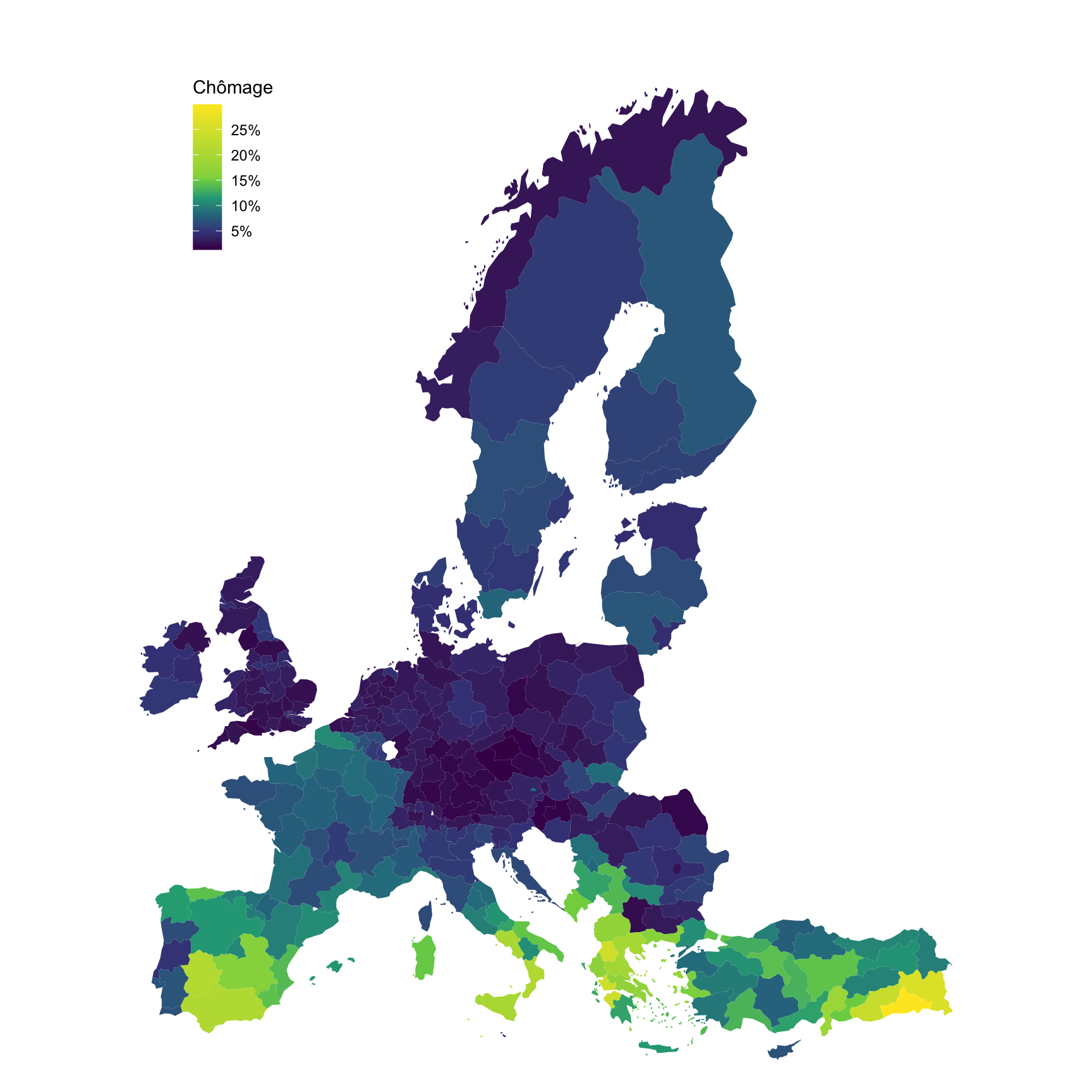
lfst_r_lfur2gac %>%
  filter(c_birth == "FOR",
         sex == "T",
         age == "Y20-64",
         nchar(geo) == 4,
         time == "2018") %>%
  right_join(europe_NUTS2, by = "geo") %>%
  filter(long >= -13.5, lat >= 33) %>%
  ggplot(., aes(x = long, y = lat, group = group, fill = values/100)) +
  geom_polygon() + coord_map() +
  scale_fill_viridis_c(na.value = "white",
                       labels = scales::percent_format(accuracy = 1),
                       breaks = 0.01*seq(0, 100, 5),
                       values = c(0, 0.1, 0.2, 0.3, 0.4, 0.5, 1)) +
  theme_void() + theme(legend.position = c(0.15, 0.85)) +
  labs(fill = "Chômage (né étranger)")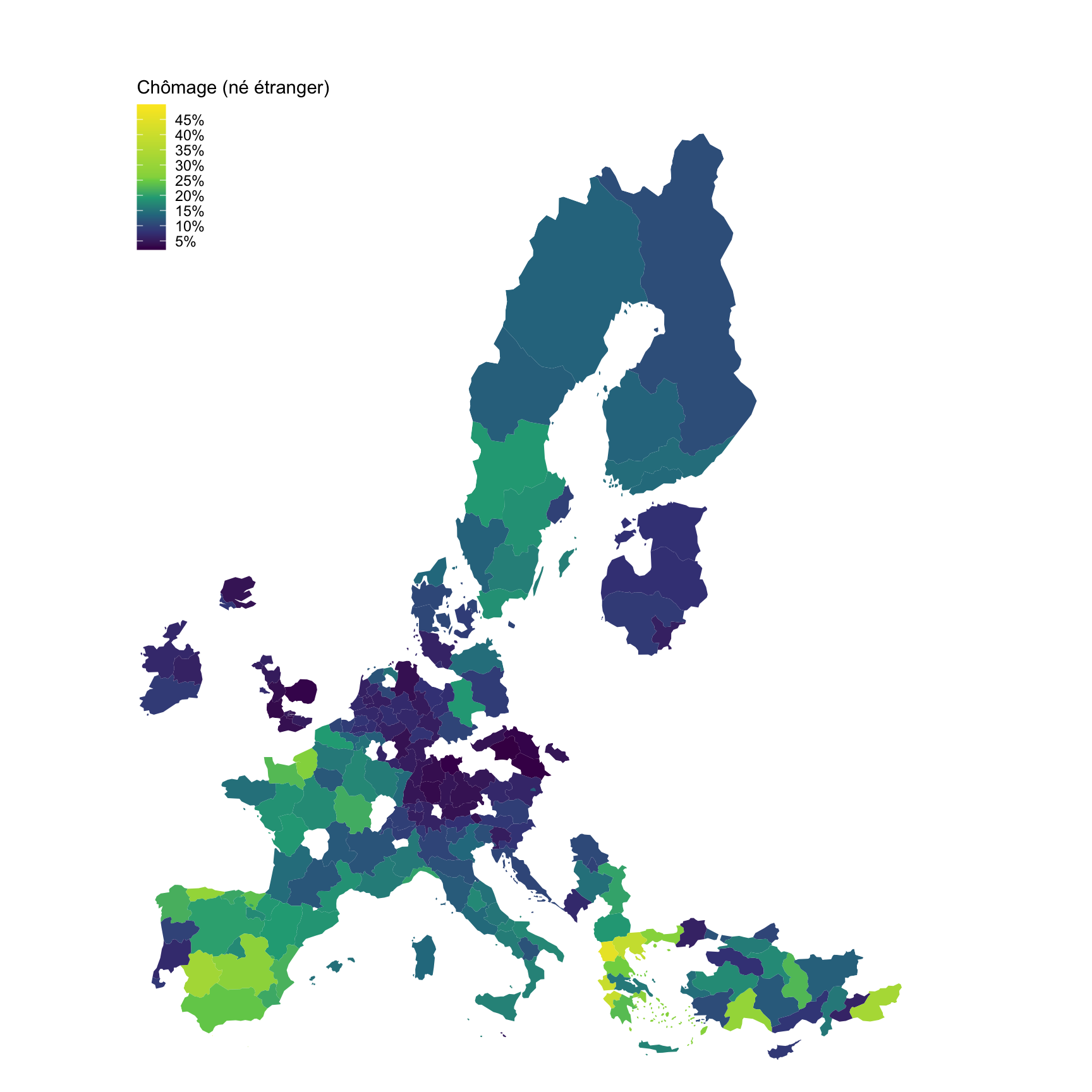
lfst_r_lfur2gac %>%
  filter(c_birth == "TOTAL",
         sex == "T",
         age == "Y25-54",
         nchar(geo) == 4,
         time == "2019") %>%
  right_join(europe_NUTS2, by = "geo") %>%
  filter(long >= -13.5, lat >= 33) %>%
  ggplot(., aes(x = long, y = lat, group = group, fill = values/100)) +
  geom_polygon() + coord_map() +
  scale_fill_viridis_c(na.value = "white",
                       labels = scales::percent_format(accuracy = 1),
                       breaks = 0.01*seq(0, 100, 5),
                       values = c(0, 0.1, 0.2, 0.3, 0.4, 0.5, 1)) +
  theme_void() + theme(legend.position = c(0.15, 0.85)) +
  labs(fill = "Chômage")