Unemployment rates by sex, age and NUTS 2 regions (%) - lfst_r_lfu3rt

Data - Eurostat

Info

Last observation: Annual: 2025 (N = 58,470)

First observation: Annual: 1999 (N = 53,968)

Last data update: 23 jul 2026, 22:15. Last compile: 24 jul 2026, 02:29

Structure

freq

isced11

sex

age

unit

geo

Unemployment Rate

lfst_r_lfu3rt %>%
  filter(time == "2015", 
         nchar(geo) == 4,
         sex == "T",
         age == "Y20-64") %>%
  
  select(geo, Geo, unemployment = values) %>%
  {if (is_html_output()) datatable(., filter = 'top', rownames = F) else .}

Unemployment - NUTS2

lfst_r_lfu3rt %>%
  filter(time == "2015", 
         nchar(geo) == 4,
         sex == "T",
         age == "Y20-64") %>%
  right_join(europe_NUTS2, by = "geo") %>%
  filter(long >= -15, lat >= 33) %>%
  ggplot(., aes(x = long, y = lat, group = group, fill = values/100)) +
  geom_polygon() + coord_map() +
  scale_fill_viridis_c(na.value = "white",
                       labels = scales::percent_format(accuracy = 1),
                       direction = -1,
                       breaks = 0.01*seq(0, 50, 5),
                       values = c(0, 0.1, 0.2, 0.3, 0.4, 0.5, 1)) +
  theme_void() + theme(legend.position = c(0.25, 0.85)) +
  labs(fill = "Unemployment (%)")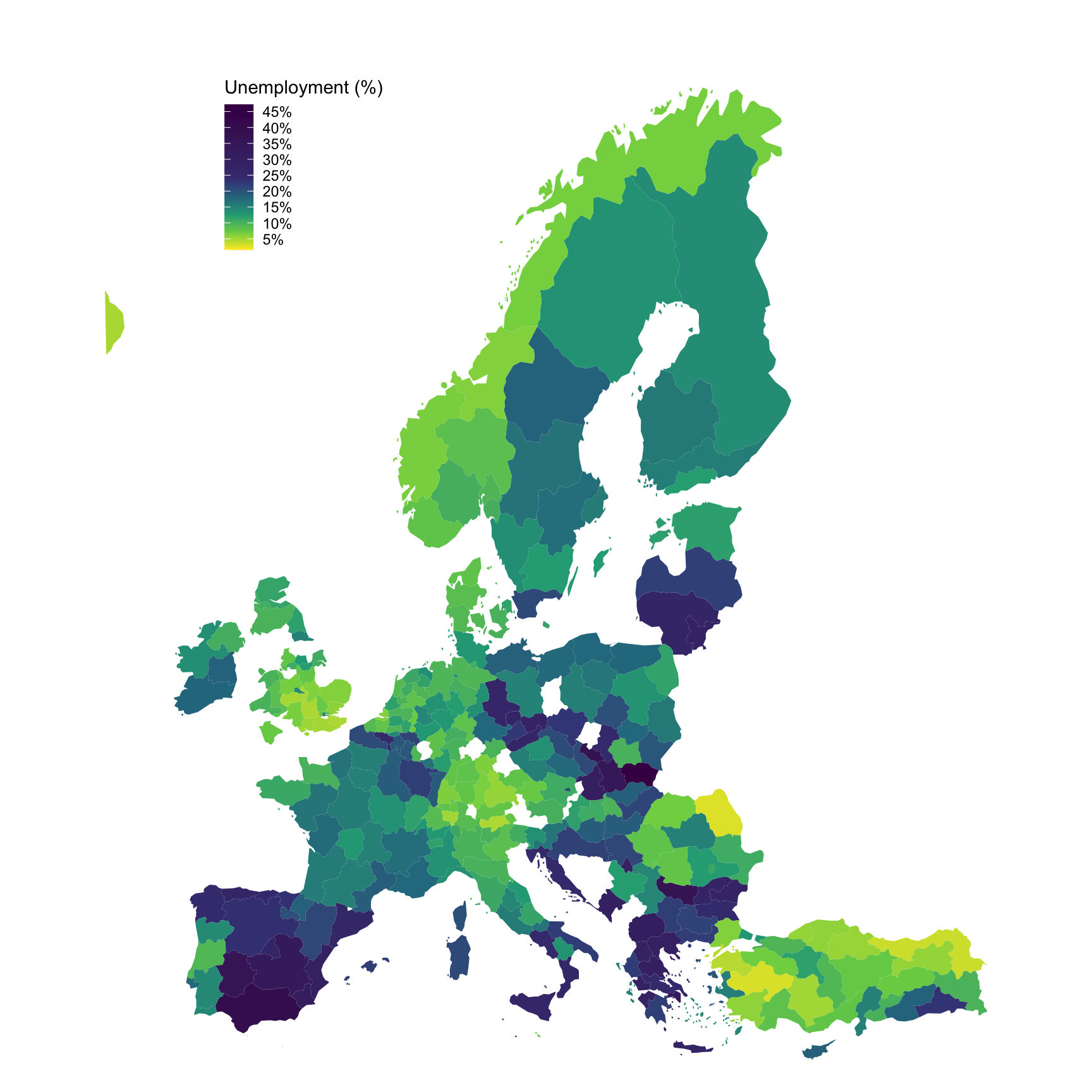

France, Germany, Italy, Spain, Poland

Unemployment Rate, Age 20-64

lfst_r_lfu3rt %>%
  filter(geo %in% c("FR", "DE", "IT", "ES", "PL"),
         sex == "T",
         age == "Y20-64",
         isced11 == "TOTAL") %>%
  year_to_date %>%
  left_join(colors, by = c("Geo" = "country")) %>%
  mutate(values = values/100) %>%
  ggplot + geom_line(aes(x = date, y = values, color = color)) +
  theme_minimal() + scale_color_identity() + add_5flags +
  scale_x_date(breaks = as.Date(paste0(seq(1999, 2100, 2), "-01-01")),
               labels = date_format("%Y")) +
  xlab("") + ylab("Unemployment rate, age 20-64") +
  scale_y_continuous(labels = scales::percent_format(accuracy = 1))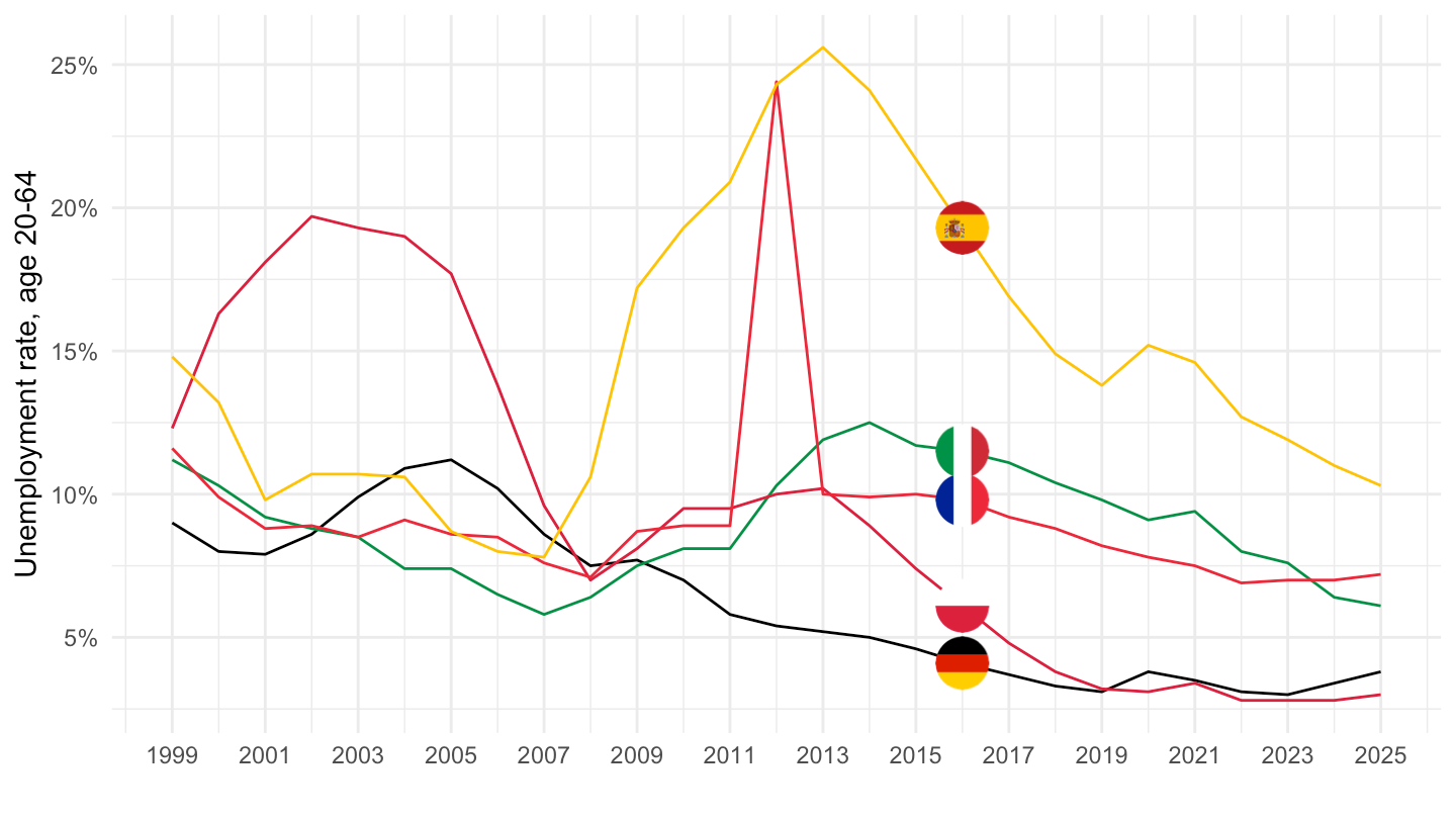

By Education Level

France

lfst_r_lfu3rt %>%
  filter(geo == "FR",
         sex == "T",
         age == "Y25-34",
         isced11 %in% c("ED0-2", "ED3_4", "ED5-8")) %>%
  year_to_date %>%
  mutate(values = values/100) %>%
  ggplot + geom_line(aes(x = date, y = values, color = Isced11)) +
  theme_minimal() +
  theme(legend.position = c(0.7, 0.75),
        legend.title = element_blank()) +
  scale_x_date(breaks = as.Date(paste0(seq(1999, 2100, 2), "-01-01")),
               labels = date_format("%Y")) +
  xlab("") + ylab("Unemployment rate, age 25-34") +
  scale_y_continuous(labels = scales::percent_format(accuracy = 1))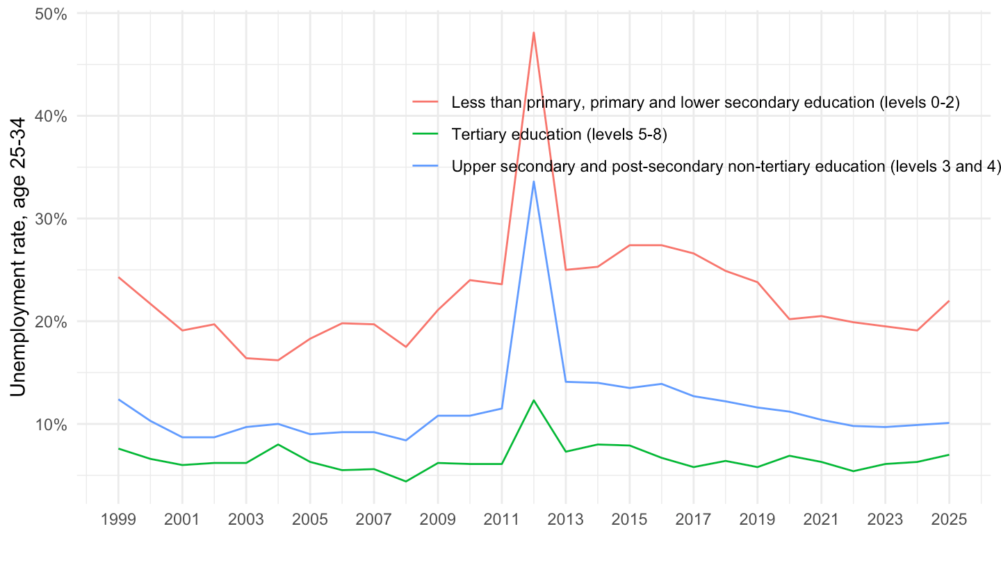

Latest Year by Country

latest_y <- lfst_r_lfu3rt %>%
  filter(nchar(geo) == 2, sex == "T", age == "Y20-64", isced11 == "TOTAL", !is.na(values)) %>%
  summarise(m = max(time)) %>%
  pull(m)

lfst_r_lfu3rt %>%
  filter(geo %in% c("FR", "DE", "IT", "ES", "PL", "NL", "PT", "SE"),
         sex %in% c("T", "F", "M"),
         age == "Y20-64",
         isced11 == "TOTAL",
         time == latest_y) %>%
  select(Geo, Sex, values) %>%
  spread(Sex, values) %>%
  print_table_conditional()

Geo	Females	Males	Total
France	7.2	7.3	7.2
Germany	3.4	4.1	3.8
Italy	6.8	5.6	6.1
Netherlands	3.5	3.2	3.3
Poland	3.3	2.8	3.0
Portugal	6.4	5.4	5.9
Spain	11.7	9.0	10.3
Sweden	7.4	7.7	7.6