
Last observation: 2025 (N = 141779)
First observation: 1999 (N = 106179)
Last data update: 11 sept. 2026, 23:01
Last compile: 04 oct. 2026, 23:25
lfst_r_lfsd2pwn |>
  filter(geo == "FR",
         age == "Y20-64",
         sex == "T",
         citizen %in% c("NAT", "FOR"),
         wstatus %in% c("EMP", "POP")) |>
  select(citizen, Citizen, wstatus, time, values) |>
  spread(wstatus, values) |>
  mutate(rate = EMP / POP) |>
  year_to_date() |>
  ggplot() + geom_line(aes(x = date, y = rate, color = Citizen)) +
  theme_minimal() +
  theme(legend.position = c(0.3, 0.15),
        legend.title = element_blank()) +
  scale_x_date(breaks = as.Date(paste0(seq(1995, 2100, 5), "-01-01")),
               labels = date_format("%Y")) +
  xlab("") + ylab("Employment rate, ages 20-64") +
  scale_y_continuous(labels = scales::percent_format(accuracy = 1))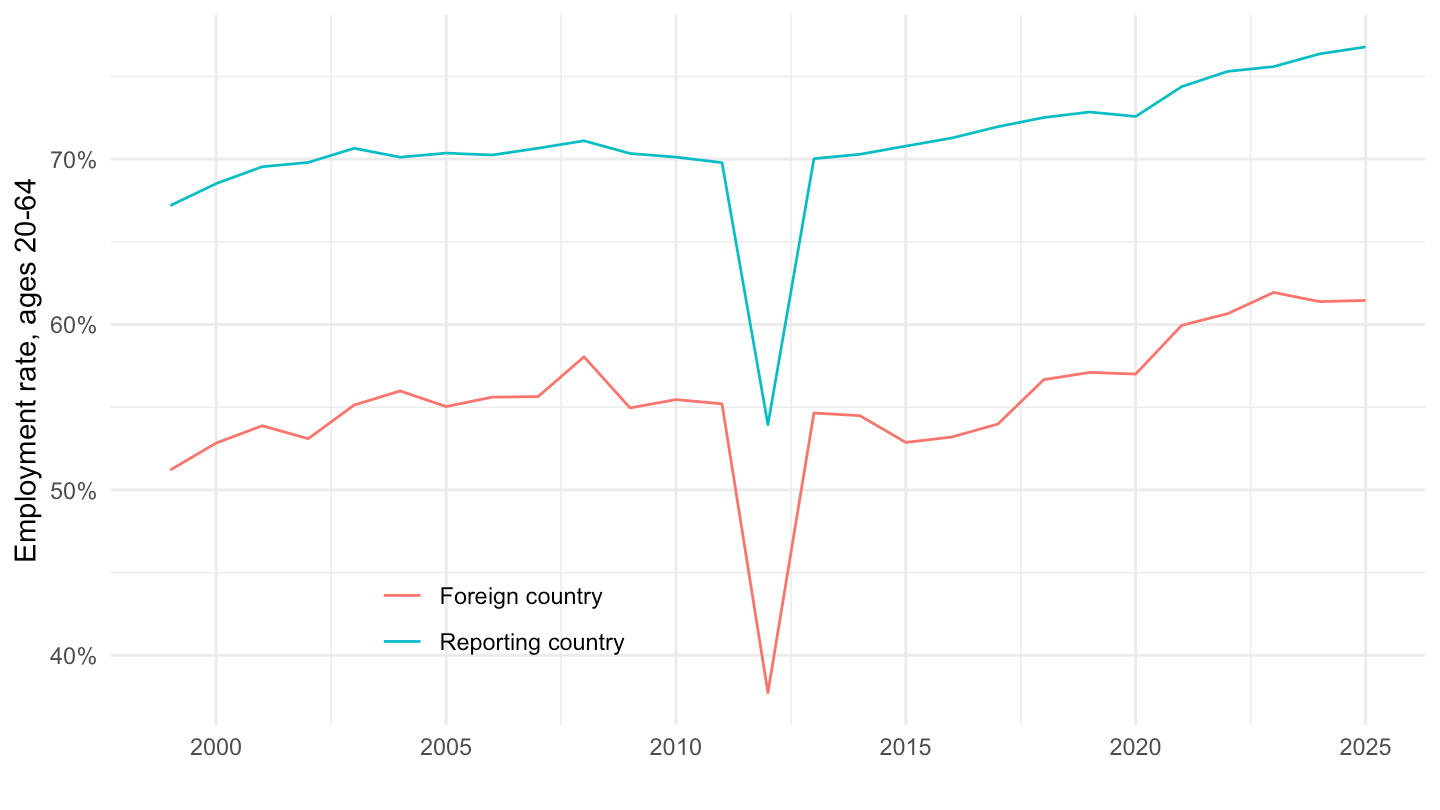
lfst_r_lfsd2pwn |>
  filter(geo %in% c("FR", "DE", "ES", "SE", "NL"),
         age == "Y20-64",
         sex == "T",
         citizen == "FOR",
         wstatus %in% c("EMP", "POP")) |>
  select(geo, Geo, wstatus, time, values) |>
  spread(wstatus, values) |>
  mutate(rate = EMP / POP) |>
  year_to_date() |>
  add_flag_color("Geo") |>
  mutate(values = rate) |>
  ggplot() + geom_line(aes(x = date, y = values, color = color)) +
  theme_minimal() + scale_color_identity() + add_flags +
  scale_x_date(breaks = as.Date(paste0(seq(1995, 2100, 5), "-01-01")),
               labels = date_format("%Y")) +
  xlab("") + ylab("Employment rate of foreign citizens, ages 20-64") +
  scale_y_continuous(labels = scales::percent_format(accuracy = 1))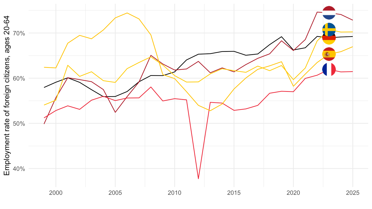
latest_y <- lfst_r_lfsd2pwn |>
  filter(age == "Y20-64", sex == "T", citizen %in% c("NAT", "FOR"),
         wstatus %in% c("EMP", "POP"), nchar(geo) == 2, !is.na(values)) |>
  summarise(m = max(time)) |>
  pull(m)

lfst_r_lfsd2pwn |>
  filter(nchar(geo) == 2,
         age == "Y20-64",
         sex == "T",
         citizen %in% c("NAT", "FOR"),
         wstatus %in% c("EMP", "POP"),
         time == latest_y) |>
  select(Geo, citizen, wstatus, values) |>
  spread(wstatus, values) |>
  mutate(rate = round(100 * EMP / POP, 1)) |>
  select(Geo, citizen, rate) |>
  spread(citizen, rate) |>
  filter(!is.na(NAT), !is.na(FOR)) |>
  mutate(gap = round(NAT - FOR, 1)) |>
  arrange(desc(gap)) |>
print_table_conditional()| Geo | FOR | NAT | gap |
|---|---|---|---|
| Bulgaria | 51.9 | 77.1 | 25.2 |
| Finland | 60.8 | 77.9 | 17.1 |
| France | 61.5 | 76.8 | 15.3 |
| Germany | 69.2 | 83.8 | 14.6 |
| Sweden | 70.2 | 83.0 | 12.8 |
| Hungary | 69.3 | 81.2 | 11.9 |
| Netherlands | 72.8 | 84.4 | 11.6 |
| Serbia | 61.8 | 71.6 | 9.8 |
| Belgium | 65.0 | 74.1 | 9.1 |
| Latvia | 70.3 | 79.2 | 8.9 |
| Austria | 71.4 | 79.6 | 8.2 |
| Switzerland | 77.7 | 84.6 | 6.9 |
| Norway | 73.7 | 80.4 | 6.7 |
| Spain | 67.0 | 73.5 | 6.5 |
| Iceland | 81.8 | 86.7 | 4.9 |
| Romania | 64.4 | 69.0 | 4.6 |
| Estonia | 78.4 | 82.4 | 4.0 |
| Cyprus | 79.3 | 82.1 | 2.8 |
| Italy | 66.8 | 67.6 | 0.8 |
| Slovenia | 77.8 | 78.4 | 0.6 |
| Portugal | 79.8 | 79.6 | -0.2 |
| Lithuania | 80.4 | 80.0 | -0.4 |
| Czechia | 83.6 | 82.8 | -0.8 |
| Greece | 72.1 | 71.0 | -1.1 |
| IE Ireland | 81.6 | 79.8 | -1.8 |
| North Macedonia | 66.5 | 63.7 | -2.8 |
| Poland | 83.8 | 78.7 | -5.1 |
| Croatia | 80.5 | 74.3 | -6.2 |
| LU Luxembourg | 77.0 | 70.0 | -7.0 |
| Slovakia | 85.9 | 78.0 | -7.9 |