Activity rates by sex, age, educational attainment level, country of birth and NUTS 2 regions - lfst_r_lfp2actrc

Data - Eurostat

Info

Last observation: Annual: 2025 (N = 108,891)

First observation: Annual: 1999 (N = 79,771)

Last data update: 23 jul 2026, 23:18. Last compile: 24 jul 2026, 02:26

Structure

freq

c_birth

isced11

age

sex

unit

geo

Education Foreign: levels 0-2

lfst_r_lfp2actrc %>%
  filter(unit == "PC",
         sex == "T",
         isced11 == "ED0-2",
         c_birth == "FOR",
         nchar(geo) == 4,
         time == "2018") %>%
  right_join(europe_NUTS2, by = "geo") %>%
  filter(long >= -13.5, lat >= 33) %>%
  ggplot(., aes(x = long, y = lat, group = group, fill = values/100)) +
  geom_polygon() + coord_map() +
  scale_fill_viridis_c(na.value = "white",
                       labels = scales::percent_format(accuracy = 1),
                       breaks = 0.01*seq(20, 100, 10),
                       values = c(0, 0.1, 0.3, 0.4, 0.5, 0.6, 1)) +
  theme_void() + theme(legend.position = c(0.15, 0.85)) +
  labs(fill = "Activity rates \nPrimary Education (%)")

Upper secondary and post-secondary non-tertiary education (levels 3 and 4)

Education Foreign: levels 3-4

lfst_r_lfp2actrc %>%
  filter(unit == "PC",
         sex == "T",
         isced11 == "ED3_4",
         c_birth == "FOR",
         nchar(geo) == 4,
         time == "2018") %>%
  right_join(europe_NUTS2, by = "geo") %>%
  filter(long >= -13.5, lat >= 33) %>%
  ggplot(., aes(x = long, y = lat, group = group, fill = values/100)) +
  geom_polygon() + coord_map() +
  scale_fill_viridis_c(na.value = "white",
                       labels = scales::percent_format(accuracy = 1),
                       breaks = 0.01*seq(20, 100, 10),
                       values = c(0, 0.5, 0.6, 0.7, 0.8, 0.9, 1)) +
  theme_void() + theme(legend.position = c(0.15, 0.85)) +
  labs(fill = "Activity rates \nSecondary Education (%)")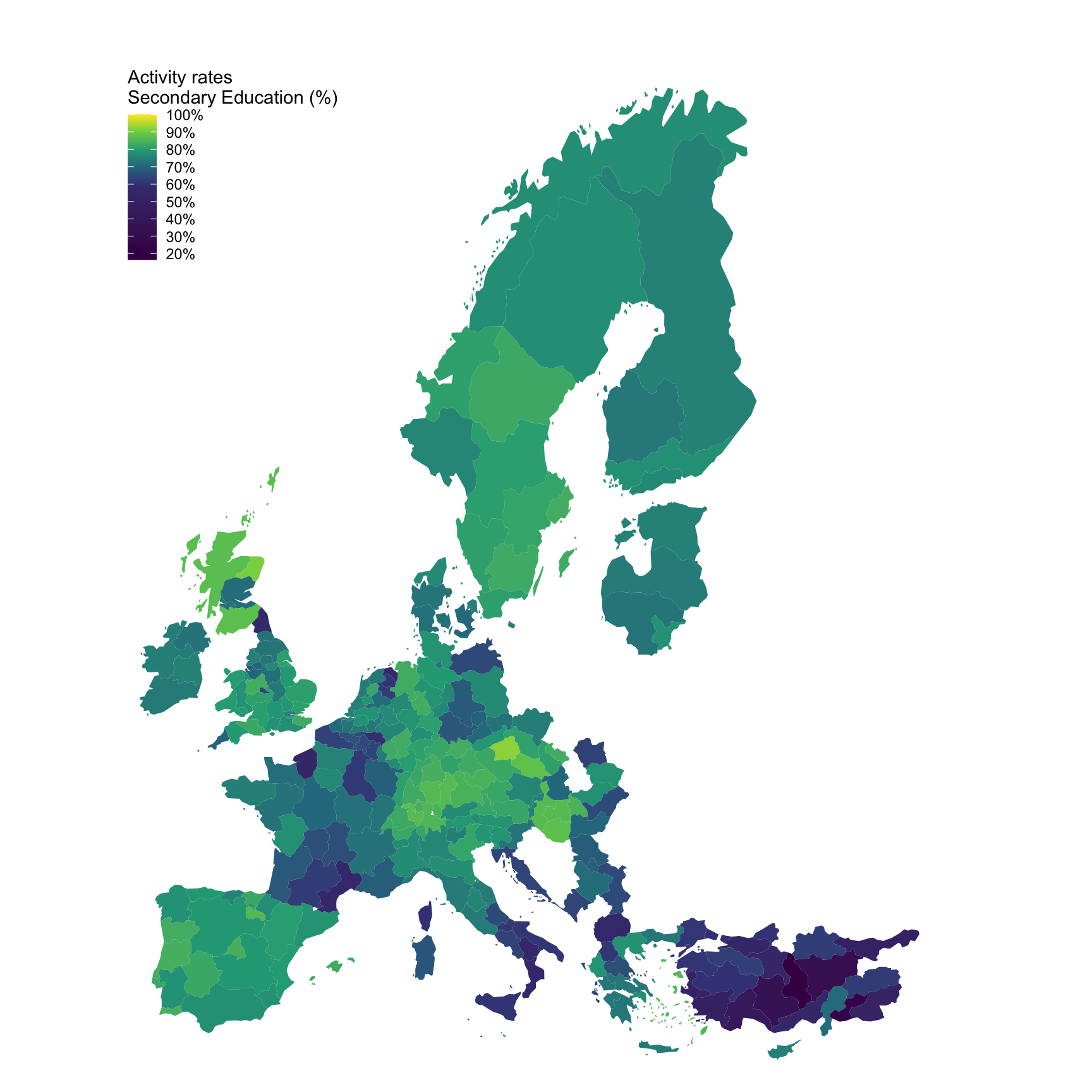

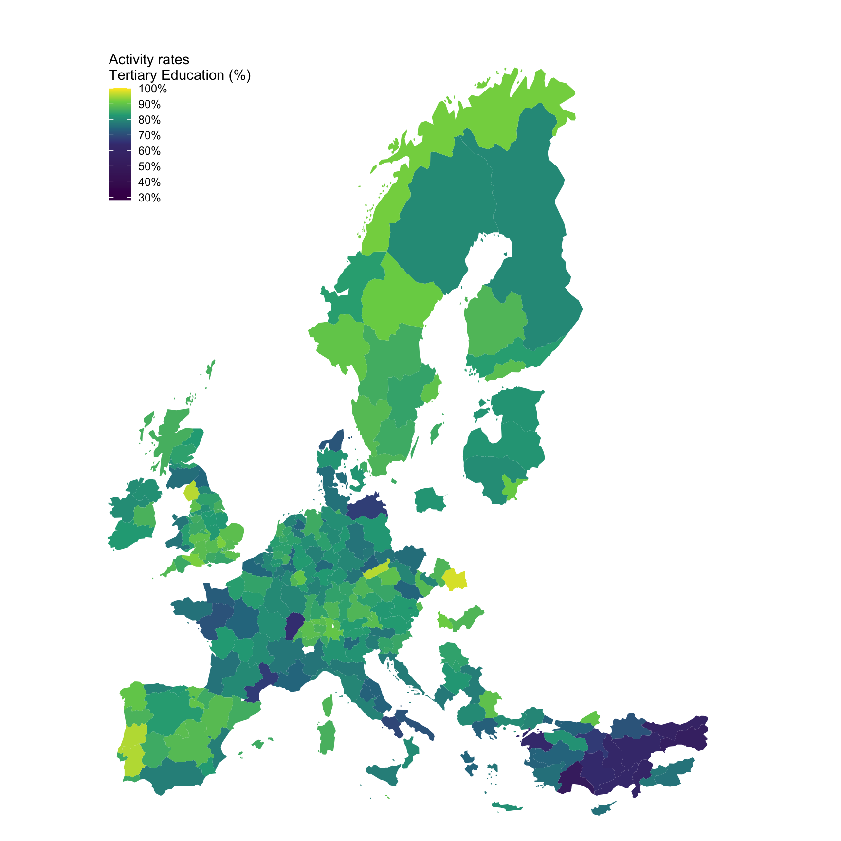
Education Foreign: levels 5-8

lfst_r_lfp2actrc %>%
  filter(unit == "PC",
         sex == "T",
         isced11 == "ED5-8",
         c_birth == "FOR",
         nchar(geo) == 4,
         time == "2018") %>%
  right_join(europe_NUTS2, by = "geo") %>%
  filter(long >= -13.5, lat >= 33) %>%
  ggplot(., aes(x = long, y = lat, group = group, fill = values/100)) +
  geom_polygon() + coord_map() +
  scale_fill_viridis_c(na.value = "white",
                       labels = scales::percent_format(accuracy = 1),
                       breaks = 0.01*seq(20, 100, 10),
                       values = c(0, 0.5, 0.6, 0.7, 0.8, 0.9, 1)) +
  theme_void() + theme(legend.position = c(0.15, 0.85)) +
  labs(fill = "Activity rates \nTertiary Education (%)")