Hours worked per week of part-time employment - lfsq_ewhun2

Data - Eurostat

Author

unit

Code

lfsq_ewhun2 %>%
  left_join(unit, by = "unit") %>%
  group_by(unit, Unit) %>%
  summarise(Nobs = n()) %>%
  arrange(-Nobs) %>%
  {if (is_html_output()) print_table(.) else .}

unit	Unit	Nobs
HR	Hour	29695364

sex

Code

lfsq_ewhun2 %>%
  left_join(sex, by = "sex") %>%
  group_by(sex, Sex) %>%
  summarise(Nobs = n()) %>%
  arrange(-Nobs) %>%
  {if (is_html_output()) print_table(.) else .}

sex	Sex	Nobs
T	Total	10593442
M	Males	9724351
F	Females	9377571

worktime

Code

lfsq_ewhun2 %>%
  left_join(worktime, by = "worktime") %>%
  group_by(worktime, Worktime) %>%
  summarise(Nobs = n()) %>%
  arrange(-Nobs) %>%
  {if (is_html_output()) print_table(.) else .}

worktime	Worktime	Nobs
TOTAL	Total	10715613
FT	Full-time	10318049
PT	Part-time	8269347
NRP	No response	392355

wstatus

Code

lfsq_ewhun2 %>%
  left_join(wstatus, by = "wstatus") %>%
  group_by(wstatus, Wstatus) %>%
  summarise(Nobs = n()) %>%
  arrange(-Nobs) %>%
  {if (is_html_output()) print_table(.) else .}

wstatus	Wstatus	Nobs
EMP	Employed persons	4862351
NCFAM	Employed persons except contributing family workers	4849974
SAL	Employees	4769968
NSAL	Employed persons except employees	3691786
SELF	Self-employed persons	3624107
SELF_NS	Self-employed persons without employees (own-account workers)	3423859
SELF_S	Self-employed persons with employees (employers)	2698917
CFAM	Contributing family workers	1638598
NRP	No response	135804

nace_r2

Code

lfsq_ewhun2 %>%
  left_join(nace_r2, by = "nace_r2") %>%
  group_by(nace_r2, Nace_r2) %>%
  summarise(Nobs = n()) %>%
  arrange(-Nobs) %>%
  {if (is_html_output()) print_table(.) else .}

nace_r2	Nace_r2	Nobs
TOTAL	Total - all NACE activities	1930006
G	Wholesale and retail trade; repair of motor vehicles and motorcycles	1709468
A	Agriculture, forestry and fishing	1685837
C	Manufacturing	1597940
M	Professional, scientific and technical activities	1591844
I	Accommodation and food service activities	1570071
S	Other service activities	1543224
F	Construction	1539606
Q	Human health and social work activities	1518680
N	Administrative and support service activities	1484101
H	Transportation and storage	1451070
R	Arts, entertainment and recreation	1451015
P	Education	1433433
J	Information and communication	1405177
K	Financial and insurance activities	1274940
L	Real estate activities	1269614
E	Water supply; sewerage, waste management and remediation activities	956835
O	Public administration and defence; compulsory social security	919566
T	Activities of households as employers; undifferentiated goods- and services-producing activities of households for own use	827296
D	Electricity, gas, steam and air conditioning supply	815342
B	Mining and quarrying	679595
NRP	No response	606644
U	Activities of extraterritorial organisations and bodies	434060

geo

Code

lfsq_ewhun2 %>%
  left_join(geo, by = "geo") %>%
  group_by(geo, Geo) %>%
  summarise(Nobs = n()) %>%
  arrange(-Nobs) %>%
  {if (is_html_output()) datatable(., filter = 'top', rownames = F) else .}

France, Germany, Portugal

Code

lfsq_ewhun2 %>%
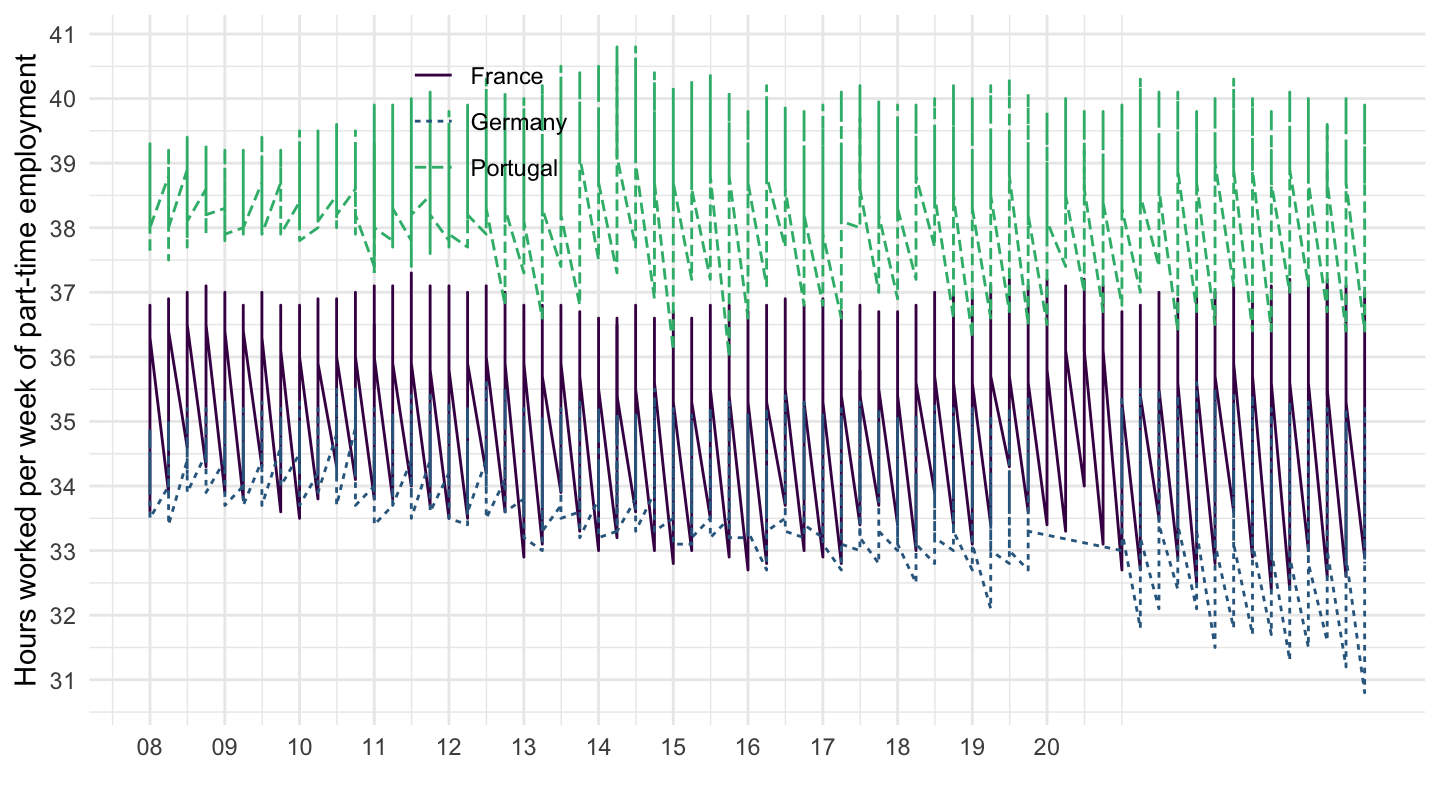
  filter(geo %in% c("FR", "DE", "PT"),
         nace_r2 == "TOTAL",
         wstatus == "SAL",
         sex == "T",
         worktime == "TOTAL") %>%
  quarter_to_date %>%
  left_join(geo, by = "geo") %>%
  ggplot + geom_line() + theme_minimal()  +
  aes(x = date, y = values, color = Geo, linetype = Geo) +
  scale_color_manual(values = viridis(4)[1:3]) +
  scale_x_date(breaks = as.Date(paste0(seq(1960, 2020, 1), "-01-01")),
               labels = date_format("%y")) +
  scale_y_continuous(breaks = seq(0, 44, 1)) +
  theme(legend.position = c(0.3, 0.85),
        legend.title = element_blank()) +
  xlab("") + ylab("Hours worked per week of part-time employment")

France, Italy, Greece

Code

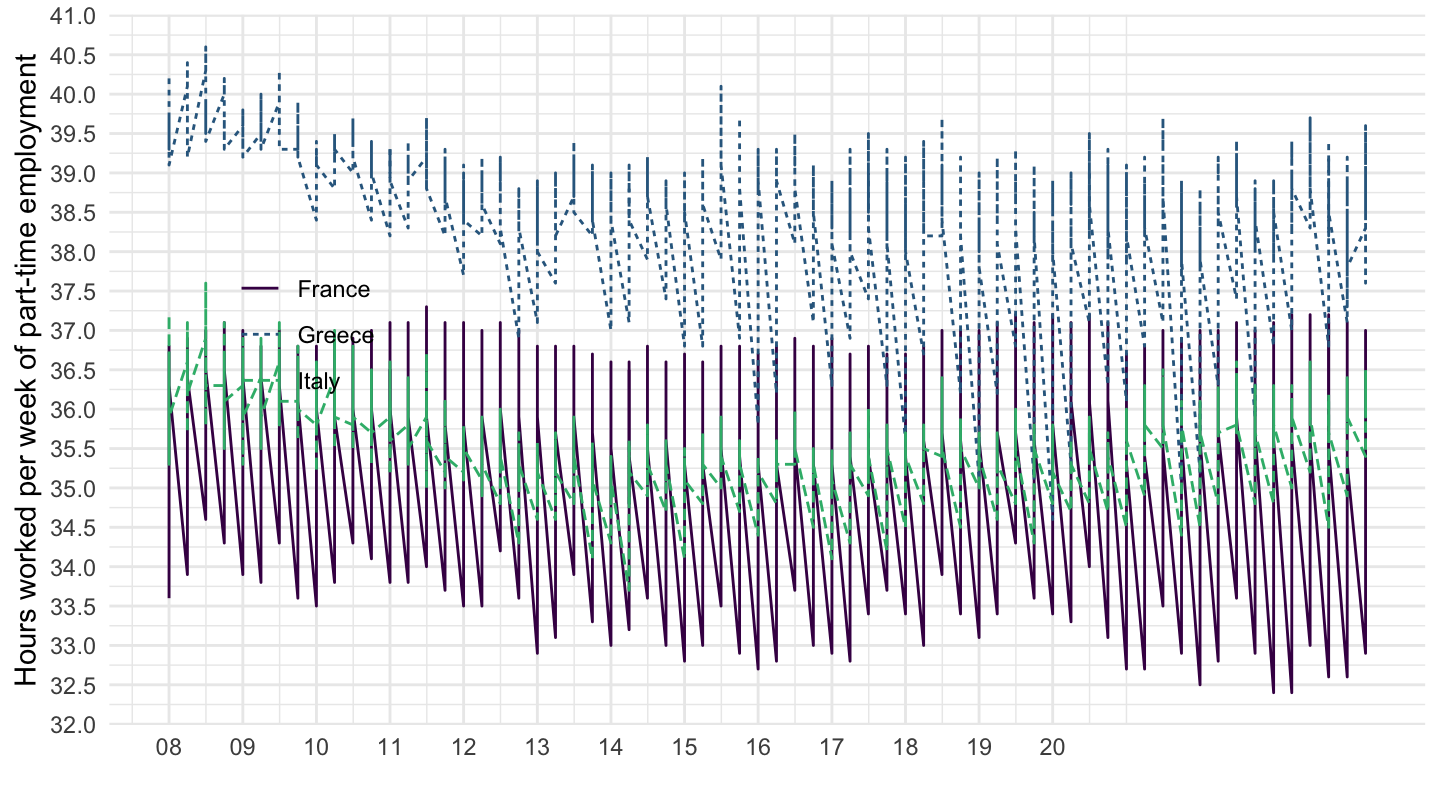
lfsq_ewhun2 %>%
  filter(geo %in% c("FR", "IT", "EL"),
         nace_r2 == "TOTAL",
         wstatus == "SAL",
         sex == "T",
         worktime == "TOTAL") %>%
  quarter_to_date %>%
  left_join(geo, by = "geo") %>%
  ggplot + geom_line() + theme_minimal()  +
  aes(x = date, y = values, color = Geo, linetype = Geo) +
  scale_color_manual(values = viridis(4)[1:3]) +
  scale_x_date(breaks = as.Date(paste0(seq(1960, 2020, 1), "-01-01")),
               labels = date_format("%y")) +
  scale_y_continuous(breaks = seq(0, 50, 0.5)) +
  theme(legend.position = c(0.15, 0.55),
        legend.title = element_blank()) +
  xlab("") + ylab("Hours worked per week of part-time employment")