Employment rates by sex, age and citizenship (%) - lfsq_ergan

Data - Eurostat

Info

Last observation: 2026Q1 (N = 13553)

First observation: 1998Q1 (N = 3223)

Last data update: 14 juil. 2026, 23:30. Last compile: 02 sept. 2026, 00:08

Structure

freq

unit

sex

age

citizen

geo

France, Germany, Portugal

25-54, Men

lfsq_ergan |>
  filter(geo %in% c("FR", "DE", "PT", "EA19"),
         sex == "M",
         citizen == "TOTAL",
         age == "Y25-54") |>
  quarter_to_date() |>
  
  mutate(values = values/100) |>
  left_join(colors, by = c("Geo" = "country")) |>
  ggplot() + geom_line() + theme_minimal()  +
  aes(x = date, y = values, color = color) +
  scale_color_identity() + add_flags +
  scale_x_date(breaks = as.Date(paste0(seq(1960, 2100, 1), "-01-01")),
               labels = date_format("%Y")) +
  scale_y_continuous(breaks = 0.01*seq(0, 100, 2),
                     labels = percent_format(a = 1)) +
  theme(legend.position = c(0.15, 0.55),
        legend.title = element_blank()) +
  xlab("") + ylab("Employment Rate, 25-54, Women (%)")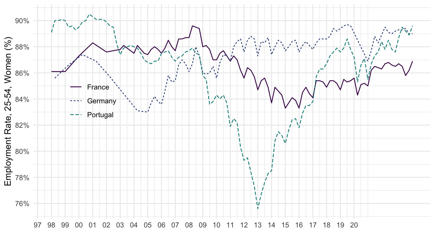

25-54, Total

lfsq_ergan |>
  filter(geo %in% c("FR", "DE", "PT", "EA19"),
         sex == "T",
         citizen == "TOTAL",
         age == "Y25-54") |>
  quarter_to_date() |>
  
  mutate(values = values/100) |>
  left_join(colors, by = c("Geo" = "country")) |>
  ggplot() + geom_line() + theme_minimal()  +
  aes(x = date, y = values, color = color) +
  scale_color_identity() + add_flags +
  scale_x_date(breaks = as.Date(paste0(seq(1960, 2100, 1), "-01-01")),
               labels = date_format("%Y")) +
  scale_y_continuous(breaks = 0.01*seq(0, 100, 2),
                     labels = percent_format(a = 1)) +
  theme(legend.position = c(0.15, 0.55),
        legend.title = element_blank()) +
  xlab("") + ylab("Employment Rate, 25-54, Total (%)")

25-54, Female

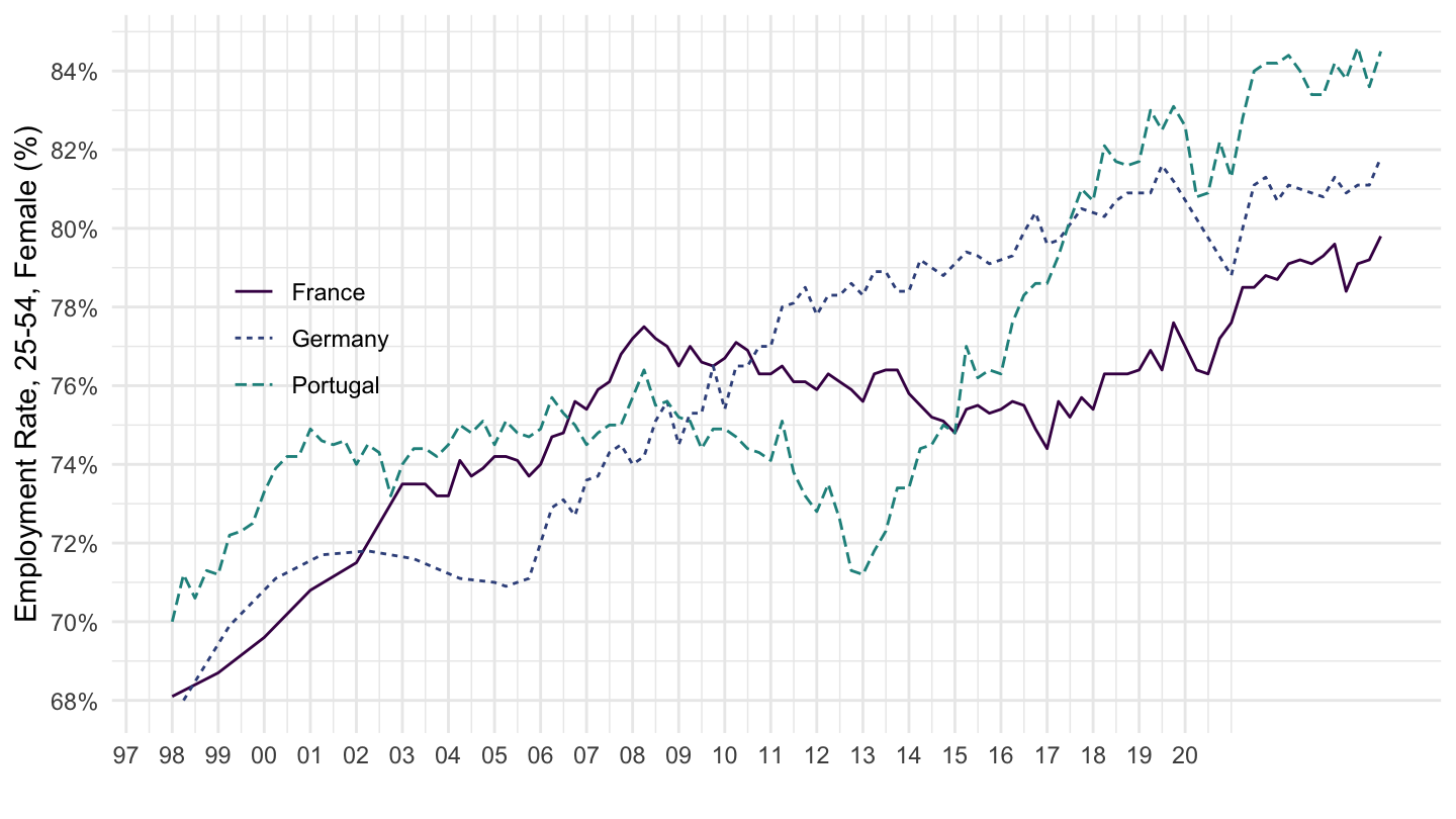
lfsq_ergan |>
  filter(geo %in% c("FR", "DE", "PT", "EA19"),
         sex == "F",
         citizen == "TOTAL",
         age == "Y25-54") |>
  quarter_to_date() |>
  
  mutate(values = values/100) |>
  left_join(colors, by = c("Geo" = "country")) |>
  ggplot() + geom_line() + theme_minimal()  +
  aes(x = date, y = values, color = color) +
  scale_color_identity() + add_flags +
  scale_x_date(breaks = as.Date(paste0(seq(1960, 2100, 1), "-01-01")),
               labels = date_format("%Y")) +
  scale_y_continuous(breaks = 0.01*seq(0, 100, 2),
                     labels = percent_format(a = 1)) +
  theme(legend.position = c(0.15, 0.55),
        legend.title = element_blank()) +
  xlab("") + ylab("Employment Rate, 25-54, Female (%)")

France, Italy, Greece

25-54, Men

lfsq_ergan |>
  filter(geo %in% c("FR", "IT", "EL", "EA19"),
         sex == "M",
         citizen == "TOTAL",
         age == "Y25-54") |>
  quarter_to_date() |>
  
  mutate(values = values/100) |>
  left_join(colors, by = c("Geo" = "country")) |>
  ggplot() + geom_line() + theme_minimal()  +
  aes(x = date, y = values, color = color) +
  scale_color_identity() + add_flags +
  scale_x_date(breaks = as.Date(paste0(seq(1960, 2100, 1), "-01-01")),
               labels = date_format("%Y")) +
  scale_y_continuous(breaks = 0.01*seq(0, 100, 5),
                     labels = percent_format(a = 1)) +
  theme(legend.position = c(0.15, 0.55),
        legend.title = element_blank()) +
  xlab("") + ylab("Employment Rate, 25-54, Men (%)")

25-54, Total

lfsq_ergan |>
  filter(geo %in% c("FR", "IT", "EL", "EA19"),
         sex == "T",
         citizen == "TOTAL",
         age == "Y25-54") |>
  quarter_to_date() |>
  
  mutate(values = values/100) |>
  left_join(colors, by = c("Geo" = "country")) |>
  ggplot() + geom_line() + theme_minimal()  +
  aes(x = date, y = values, color = color) +
  scale_color_identity() + add_flags +
  scale_x_date(breaks = as.Date(paste0(seq(1960, 2100, 1), "-01-01")),
               labels = date_format("%Y")) +
  scale_y_continuous(breaks = 0.01*seq(0, 100, 5),
                     labels = percent_format(a = 1)) +
  theme(legend.position = c(0.15, 0.55),
        legend.title = element_blank()) +
  xlab("") + ylab("Employment Rate, 25-54, Total (%)")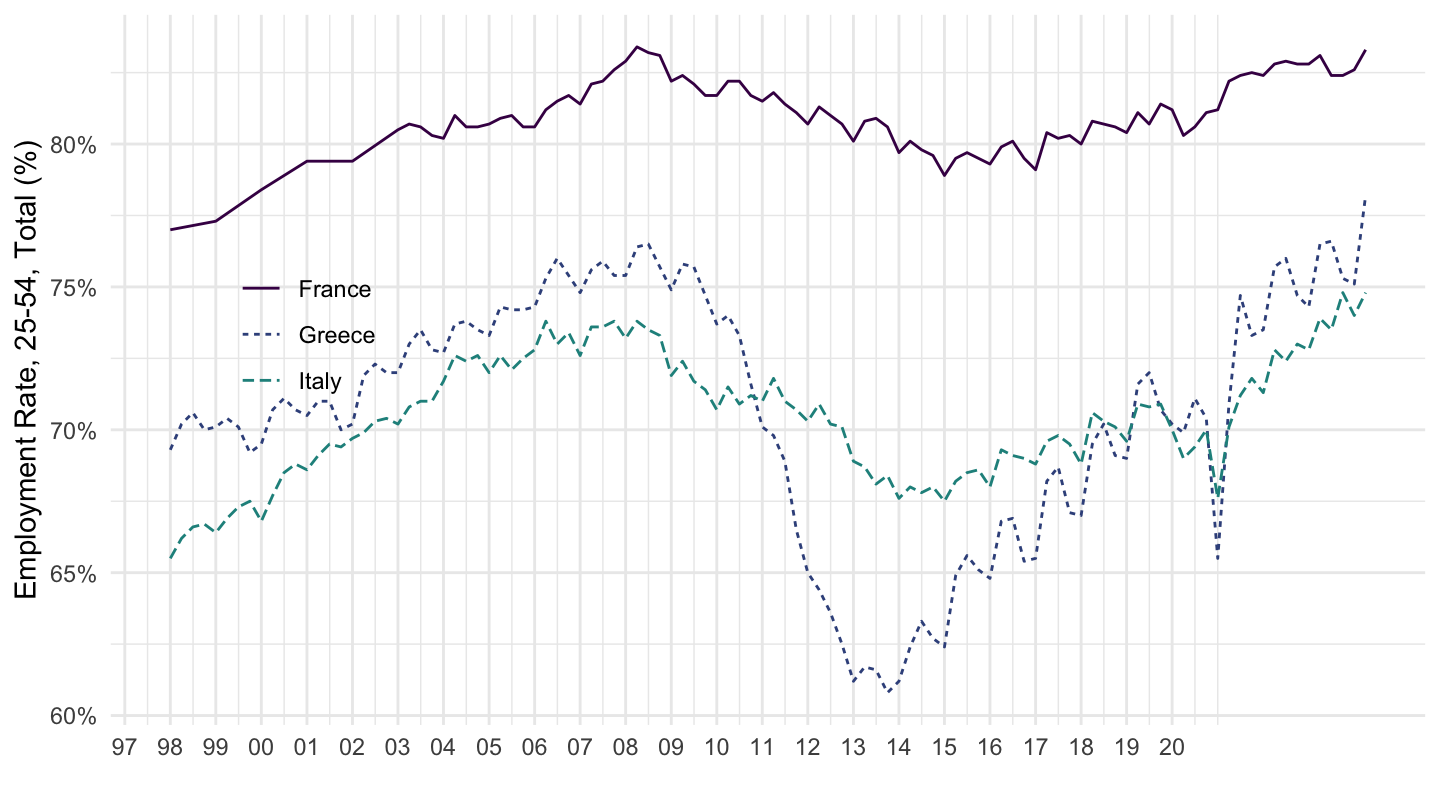

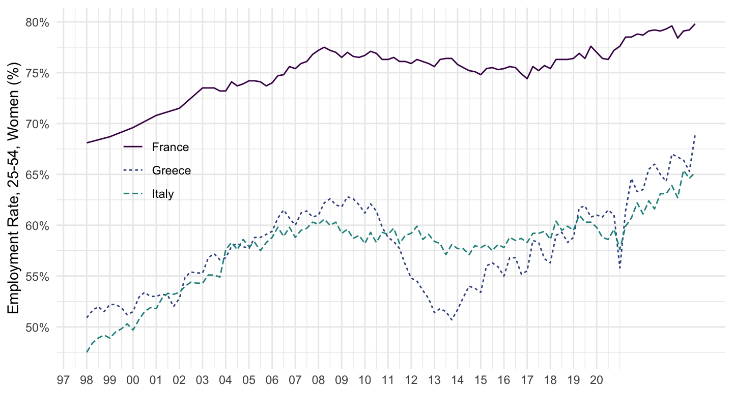
25-54, Women

lfsq_ergan |>
  filter(geo %in% c("FR", "IT", "EL", "EA19"),
         sex == "F",
         citizen == "TOTAL",
         age == "Y25-54") |>
  quarter_to_date() |>
  
  mutate(values = values/100) |>
  left_join(colors, by = c("Geo" = "country")) |>
  ggplot() + geom_line() + theme_minimal()  +
  aes(x = date, y = values, color = color) +
  scale_color_identity() + add_flags +
  scale_x_date(breaks = as.Date(paste0(seq(1960, 2100, 1), "-01-01")),
               labels = date_format("%Y")) +
  scale_y_continuous(breaks = 0.01*seq(0, 100, 5),
                     labels = percent_format(a = 1)) +
  theme(legend.position = c(0.15, 0.55),
        legend.title = element_blank()) +
  xlab("") + ylab("Employment Rate, 25-54, Women (%)")